Explanatory and Response Variables, Correlation (2.1)
Summary
TLDRThis video script explores the concepts of explanatory and response variables, as well as correlation, in the context of statistical analysis. It explains how to use time plots and scatter plots to visualize the relationship between two variables, emphasizing the importance of identifying which variable is explanatory and which is responsive. The script delves into how correlation, denoted as 'R', measures both the direction and strength of a linear relationship between variables, and provides a step-by-step guide on calculating it using a formula. It concludes with a cautionary note on the potential for visual deception when interpreting correlation from scatter plots alone.
Takeaways
- 📊 Descriptive statistics like histograms, stem plots, and box plots are used to describe a single variable, while time plots and scatter plots are used to show relationships between two variables.
- 🌳 In a time plot, one variable is the explanatory variable (e.g., age of a tree), and the other is the response variable (e.g., tree height), indicating a cause-and-effect relationship.
- 📈 A scatter plot represents the values of two quantitative variables from the same population, with the explanatory variable typically on the x-axis and the response variable on the y-axis.
- 🔄 The terms 'explanatory variable' and 'response variable' can be used interchangeably with 'independent variable' and 'dependent variable', respectively.
- ⚠️ Not all data sets have an explanatory and response variable; some variables are unrelated and do not have a cause-and-effect relationship.
- 🔍 Correlation, denoted as R, measures the direction and strength of a linear relationship between two quantitative variables, independent of whether they are explanatory or response variables.
- ⬆️ A positive correlation indicates an upward slope in the data set, while a negative correlation indicates a downward slope.
- 🔢 The value of R ranges from -1 to 1, with -1 indicating a perfect negative correlation, 1 indicating a perfect positive correlation, and 0 indicating no correlation.
- 📝 The formula for calculating correlation involves the means, standard deviations, and the sum of the products of the differences from the means of the paired variables.
- 📚 To calculate correlation, gather data, create a table, calculate means and standard deviations, and apply the formula to find the correlation coefficient.
- 👀 Visual inspection of a scatter plot can be misleading; the actual value of R should be calculated and interpreted numerically rather than relying on visual assessment alone.
Q & A
What is the purpose of using histograms, stem plots, and box plots?
-Histograms, stem plots, and box plots are used to describe one variable. They help in understanding the distribution and characteristics of a single dataset.
How can we compare two different populations with respect to the same variable?
-We can use back-to-back stem plots and side-by-side box plots to compare two different populations with respect to the same variable, which helps in visualizing the differences and similarities between the two groups.
What is the difference between a response variable and an explanatory variable?
-A response variable measures the outcome of a study, while an explanatory variable explains the outcome. For example, in a study about trees, the height of the tree is the response variable, and the age of the tree is the explanatory variable.
Why is a time plot used to show the relationship between two variables?
-A time plot is used to show the relationship between two variables when there is a temporal relationship, where one variable changes in response to the other over time.
What is a scatter plot and how is it different from a time plot?
-A scatter plot is a graphical representation of two quantitative variables from the same population, where each dot represents an individual's values for both variables. Unlike a time plot, a scatter plot does not necessarily have time on the x-axis.
Why is the explanatory variable usually plotted on the x-axis and the response variable on the y-axis?
-The explanatory variable is plotted on the x-axis and the response variable on the y-axis because it represents the independent and dependent variables, respectively, with the explanatory variable influencing the response variable.
What is the role of correlation in data analysis?
-Correlation, denoted as R, measures the direction and strength of a linear relationship between two quantitative variables. It helps in understanding how two variables move in relation to each other.
How is the direction of a data set's slope related to the value of R in correlation?
-If a data set has an upward slope, R is positive, indicating a positive correlation. If it has a downward slope, R is negative, indicating a negative correlation. A perfect straight line slope results in R being either +1 or -1, representing perfect positive or negative correlation.
What does the value of R equal to 0 indicate in terms of correlation?
-When R is equal to 0, it indicates that there is no correlation, meaning there is no linear relationship between the two variables.
How can we calculate the correlation between two variables?
-Correlation can be calculated using a formula that involves the means, standard deviations, and the sum of the products of the differences from the means for each variable. The formula is more complex than it appears but follows a systematic process of calculation.
Why is it misleading to interpret correlation based solely on the visual appearance of a scatter plot?
-Interpreting correlation based on the visual appearance of a scatter plot can be misleading because different scales can make the relationship appear stronger or weaker. The actual numerical value of R is needed to accurately determine the strength and direction of the correlation.
Outlines

This section is available to paid users only. Please upgrade to access this part.
Upgrade NowMindmap

This section is available to paid users only. Please upgrade to access this part.
Upgrade NowKeywords

This section is available to paid users only. Please upgrade to access this part.
Upgrade NowHighlights

This section is available to paid users only. Please upgrade to access this part.
Upgrade NowTranscripts

This section is available to paid users only. Please upgrade to access this part.
Upgrade NowBrowse More Related Video
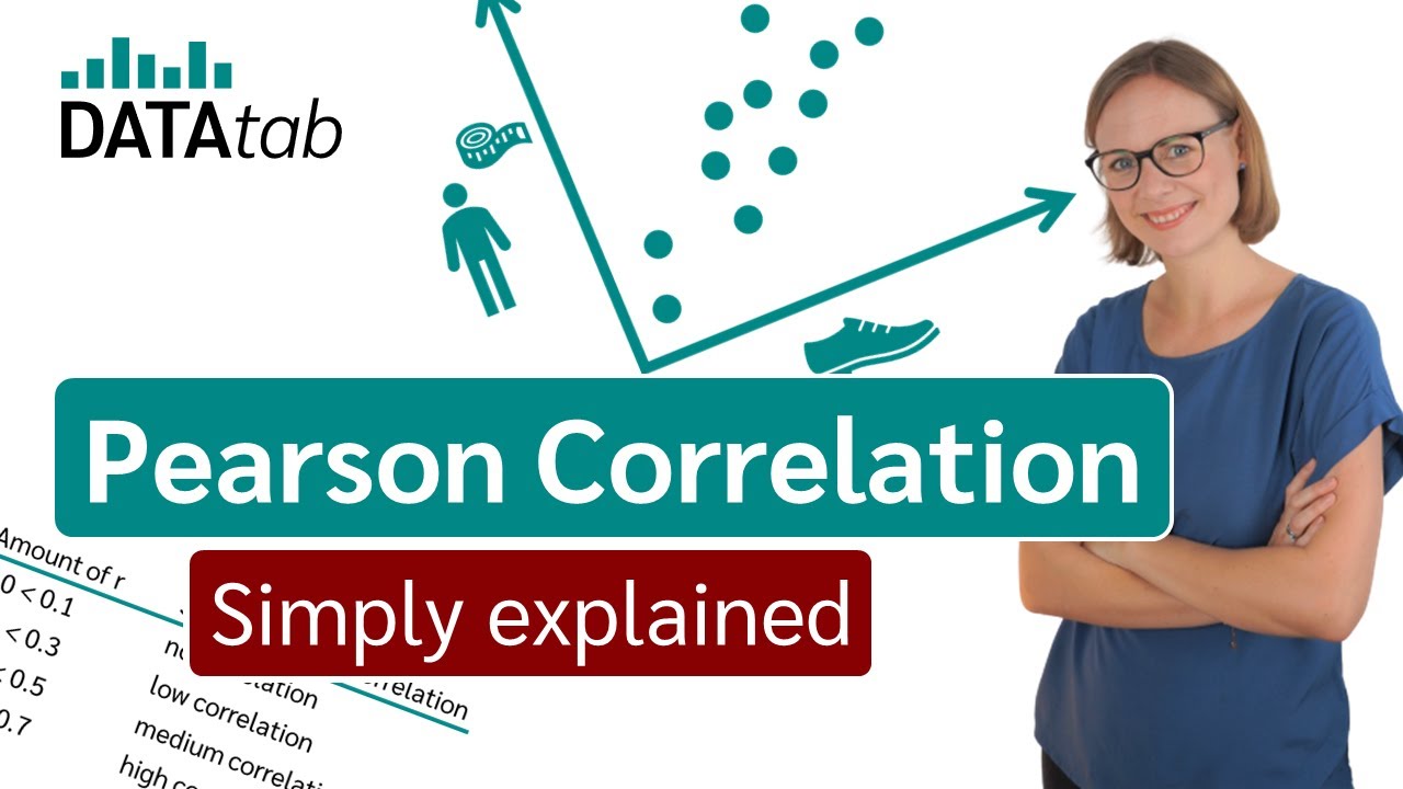
Pearson correlation [Simply explained]

Statistik Teori pertemuan ke ~ 9 Korelasi dan Regresi

Analisis Regresi Sederhana - Statistika Ekonomi dan Bisnis Lanjutan (Statistik 2) | E-Learning STA
一夜。統計學:相關分析
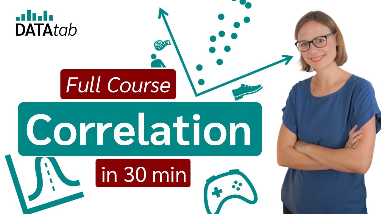
Correlation Analysis - Full Course in 30 min
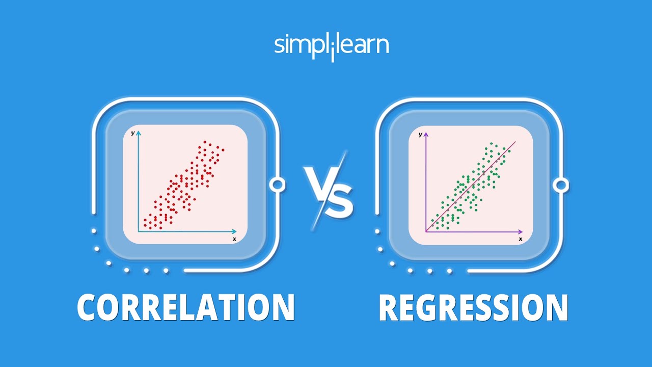
Correlation vs Regression | Difference Between Correlation and Regression | Statistics | Simplilearn
5.0 / 5 (0 votes)