Excel Conditional Formatting in Depth
Summary
TLDRThis tutorial explores conditional formatting in Microsoft Excel, demonstrating how to visually represent data based on specific conditions using two spreadsheets. It covers highlighting cells, top/bottom rules, data bars, color scales, and icon sets, offering a comprehensive guide to making spreadsheets more informative and visually appealing.
Takeaways
- π Conditional formatting in Microsoft Excel allows you to change how data looks based on certain conditions.
- π You can find conditional formatting in the Home tab under the Styles group.
- π° Highlighting cells with values greater than a specified number can help visually represent important data, such as the most valuable DVDs in an inventory.
- π You can customize the formatting rules to change the fill color and text color, and preview changes before applying them.
- π« It's important to clear rules from selected cells if you don't want certain text, like headers, to be formatted.
- π Conditional formatting can automatically apply to new data if you apply it to an entire column or row, rather than just a selected range.
- π Top/bottom rules can be used to highlight the highest or lowest values in a dataset, and you can manage and edit these rules as needed.
- π Data bars provide a visual representation of data by showing bars in cells that grow with the value, making it easy to compare values at a glance.
- π Color scales offer a gradient of colors to represent data values, helping to quickly identify trends and patterns.
- π·οΈ Icon sets can be used to display icons in cells based on the data value, providing another visual method to understand data distribution.
- π More advanced options and custom formats can be explored in conditional formatting to further enhance data visualization and understanding.
Q & A
What is the main topic of the tutorial?
-The main topic of the tutorial is conditional formatting in Microsoft Excel.
What are the two spreadsheets used in the video?
-The two spreadsheets used in the video are a movie inventory spreadsheet and a spreadsheet of financial data.
Where can conditional formatting be found in Excel?
-Conditional formatting can be found on the Home tab, under the Styles group in Excel.
What is the purpose of using conditional formatting?
-The purpose of using conditional formatting is to change how data looks in the spreadsheet based on certain conditions, making it easier to identify and analyze specific data points.
How can you highlight cells with values greater than a certain number using conditional formatting?
-You can highlight cells with values greater than a certain number by selecting the cells, going to the Home tab, clicking on conditional formatting, choosing 'Highlight cells rules', and then specifying the condition and the formatting style.
What is the issue with highlighting the word 'value' in the spreadsheet?
-The issue with highlighting the word 'value' is that it is not a data point and should not be formatted based on the condition set for numerical values.
How can you clear conditional formatting from selected cells?
-You can clear conditional formatting from selected cells by right-clicking on the cells, going to 'Conditional Formatting', and choosing 'Clear Rules' from the 'Selected Cells'.
What are some examples of conditional formatting rules that can be applied?
-Examples of conditional formatting rules include highlighting cells greater than a certain value, less than a certain value, between two numbers, equal to a specific number, or containing certain text.
What are data bars and how do they help in visualizing data?
-Data bars are a visual representation of data where the size of the bar inside a cell corresponds to the value of the data. They help in easily comparing values at a glance by showing the relative size of the data points.
How can you customize the appearance of conditional formatting rules?
-You can customize the appearance of conditional formatting rules by choosing different colors, patterns, borders, and font styles through the 'Fill', 'Font', and 'Border' options in the conditional formatting menu.
What is the difference between data bars and color scales in conditional formatting?
-Data bars represent data with visual bars inside the cells, while color scales use a gradient of colors to indicate the value of the data, with darker colors representing lower values and lighter colors representing higher values.
What are icon sets in conditional formatting and how do they work?
-Icon sets in conditional formatting are symbols that appear in each cell based on the value of the data. They help in quickly identifying the relative value of data points by using visual symbols like arrows, traffic lights, or stars.
How can you adjust the thresholds for icon sets in conditional formatting?
-You can adjust the thresholds for icon sets by going to 'More Rules', selecting 'Edit Rule', and changing the percentage or specific values that determine when each icon appears.
Outlines
π Introduction to Conditional Formatting in Excel
This paragraph introduces the concept of conditional formatting in Microsoft Excel. The speaker uses two spreadsheets: a movie inventory and a financial data spreadsheet, to demonstrate how conditional formatting can be applied. The purpose is to change the appearance of data based on certain conditions, making it easier to identify and visualize specific information. The Home tab's Styles group is highlighted as the location to access conditional formatting options. The paragraph sets the stage for exploring various conditional formatting rules and their applications.
π Highlighting Cells with Specific Data
In this segment, the speaker discusses how to use conditional formatting to highlight cells based on specific criteria. Examples include highlighting cells with values greater than a certain number, such as 999, and changing the formatting to a green fill with dark green text. The speaker also demonstrates how to correct mistakes, such as highlighting non-numeric text, by clearing rules from selected cells. The importance of applying conditional formatting to entire columns or rows for consistency with new data is emphasized. Additionally, the paragraph covers highlighting cells with text containing specific words, setting custom formats, and identifying duplicate or unique values.
π Top/Bottom Rules and Data Bars
The speaker transitions to discussing top/bottom rules in conditional formatting, using a financial data spreadsheet as an example. The focus is on how to highlight the top or bottom values in a range, such as the top 10 items. The speaker also shows how to manage and edit existing rules, and how to apply different percentages or values for highlighting. Data bars are introduced as a visual way to represent data, with options for color and style. The segment covers how to customize data bars to show only the bars without the numerical values, providing a clear visual comparison of data.
π¨ Color Scales, Icon Sets, and Customization
This paragraph delves into color scales and icon sets in conditional formatting. Color scales provide a visual representation of data with a gradient of colors, while icon sets use symbols to indicate data values. The speaker demonstrates how to choose different color schemes and icon types, and how to adjust the number of icons to fit the data distribution. The paragraph also covers how to customize the cutoff values for icons and how to adjust the width of columns to accommodate icons. The speaker concludes by encouraging viewers to explore advanced options and customization possibilities in conditional formatting.
π£ Conclusion and Future Content Preview
In the final paragraph, the speaker wraps up the tutorial on conditional formatting and invites viewers to like, share, and subscribe for more content. The speaker also mentions plans for an advanced video on highlighting entire rows based on conditional formatting, providing a sneak peek into future content. Additionally, the speaker encourages viewers to connect on social media and become supporters through Patreon, with links provided in the video description.
Mindmap
Keywords
π‘Conditional Formatting
π‘Movie Inventory Spreadsheet
π‘Financial Data Spreadsheet
π‘Highlight Cells Rules
π‘Data Bars
π‘Color Scales
π‘Icon Sets
π‘Top/Bottom Rules
π‘Unique/Duplicate Values
π‘Custom Formats
Highlights
Introduction to conditional formatting in Microsoft Excel.
Using two different spreadsheets: a movie inventory and a financial data spreadsheet.
Conditional formatting changes the appearance of data based on certain conditions.
Accessing conditional formatting in the Home tab under the Styles group.
Highlighting cells with values greater than a specified number using 'Highlight Cells Rules'.
Customizing the formatting style, such as changing to a green fill with dark green text.
Automatically formatting new data in a selected range.
Clearing rules from selected cells to avoid unwanted formatting.
Highlighting cells with values less than a certain number.
Highlighting text that contains specific information, such as the word 'star'.
Creating custom formats for conditional formatting.
Using 'Highlight Cells Rules' to find duplicate values.
Formatting the top or bottom values in a range with 'Top/Bottom Rules'.
Adjusting the number of top or bottom values to highlight, such as top 10 to top 60.
Using data bars to visually represent data with different colors and styles.
Hiding cell values and showing only data bars for a presentation.
Choosing color scales to visually represent data with a gradient of colors.
Using icon sets to represent data values with symbols like arrows, traffic lights, or flags.
Customizing icon set cutoffs to fit specific data distribution needs.
Upcoming advanced video on highlighting entire rows based on conditional formatting.
Invitation to support the YouTube channel through Patreon.
Transcripts
in this tutorial we're gonna take a
close look at conditional formatting in
Microsoft Excel and for this video we're
going to use two different spreadsheets
this is the movie inventory spreadsheet
that I used in some of my previous
videos including the beginners guide to
Microsoft Excel if you haven't watched
that you definitely should but this is
just an inventory of movies that I own
and some information about them I will
also be using this spreadsheet this is a
spreadsheet of a lot of financial data
and it's a good example of the kinds of
huge spreadsheets with lots and lots of
data that a lot of times businesses have
and use so let's jump right in to
conditional formatting what it is and
how to use it so in my beginners guide
to Microsoft Excel I gave a little bit
of a sneak peek into conditional
formatting let's talk about what it is
conditional formatting is a tool that
gives us the opportunity to change how
data looks in the spreadsheet it formats
the data in the spreadsheet based upon
certain conditions that's why it's
called conditional formatting and you'll
find conditional formatting on the Home
tab home ribbon in the Styles group so
let's look at some of the things it's
capable of doing for us let's say I
would like a visual representation of
the DVDs that are worth the most right
now so I can look here at the value
column column D and I can just eyeball
this and see which ones are more
valuable right now now of course I could
also apply a filter that would filter
out the cheaper less valuable DVDs but
that would hide data and let's say I'd
like to be able to see all of the data
but be able to add a glance see which
ones are more valuable so the way to do
that is to select column D in this case
and go to the Home tab home ribbon
Styles group and click conditional
formatting now there are several
different options that appear and this
is what we're gonna look at in this
video what do all of these options do
for us so let's start first with the top
option highlight cells rules so I would
like to highlight cells that
numbers that are greater than a certain
number and I'm gonna put as the number
nine point nine nine so greater than
nine ninety nine and I just typed that
right in this box here now next to that
it says with light red fill with dark
red text so format cells that are
greater than 999 with red basically well
I would like to change that in general I
think green represents money in a lot of
cases and so I would like to say green
fill with dark green text I click there
and I get a sneak preview of what it
will look like and if I like it I click
OK if I don't I can click cancel but
I'll click OK so you can see what that
did it automatically changed the format
of these particular cells because 14 is
greater than nine point nine nine so is
15 so is 10 so those are all highlighted
in green now notice what else is
highlighted in green the word value
somehow the word value is greater than
nine point nine nine and this is not
really what I wanted I don't want the
word value in green so how can I fix
that well what I would do is I would
just click on the word value go to
conditional formatting and clear rules
from selected cells I could clear them
from the entire sheet but then I would
lose the formatting that I do want this
down here so I'm just gonna clear rules
from selected cells and now that's
exactly what I wanted to do now some of
you might be wondering why didn't I just
click and drag and not include the word
value in the spreadsheet range that I
applied to conditional formatting - well
the reason I didn't do that is because
if I put in new data notice that it's
automatically formatted correctly but
that would not be the case if I had just
clicked and dragged it to select a range
that's why it's better in most cases to
click an entire column or if you want
even a row and apply the conditional
formatting to all of the information and
then just click and clear the rules from
the selected cells so hopefully that
makes sense now in a spreadsheet this
small you can see that it is pretty
useful it does highlight those more
valuable items for me but imagine
a spreadsheet that was much much bigger
conditional formatting can be even more
useful in these cases I think let's try
a second example of how we can use
conditional formatting I'm gonna go here
to units sold and click the entire
column E and I'll go to conditional
formatting and I just want to quickly
show you that in addition to greater
than you can also do less than so I
could highlight cells that have data
that's less than this number and I can
change that number I can also highlight
data that is between two numbers that's
equal to a specific number I can also
highlight text that contains certain
information so for example let's jump
back to my movie inventory and I will
select column a choose conditional
formatting highlight cells rules and I
want to highlight text that contains the
word star and I want to highlight it in
green and you can see how that works now
while I'm at it I want to show you that
you can also set up your own custom
formats so if you're not happy with the
built-in options for formats you can
just create your own so for example I
can go to fill and I can say I would
like it to be filled in orange the
pattern color I would like it to be a
little bit lighter orange what patterns
style hmm how about this and I'll put in
a border what about the font I would
like it to be bold and the color of the
font I would like it to not be automatic
maybe I'd like it to be dark green and
then just click OK so as you can see you
can design your own personal custom
formats that change how the data looks
on the screen in most cases though I
typically just use yellow green and red
the defaults that are here ok notice
that you can also use highlight cells
rules to find an occurring date and also
to find duplicate values so in this case
it's finding every number that is
repeated somewhere else in this column
it is possible to also do a similar
thing but look not for duplicates but
for unique values
so as you can see here I just went to
highlight cells rules more rules and
here it says format only unique or
duplicate values and then you change it
from duplicate to unique you can set up
the format that you want it to do and
then click OK so this is showing cells
that have unique information in this
column ok so this conditional formatting
highlight cells rules category has lots
of great options for us to help us
format data the way we want it to look
next let's look at top/bottom rules and
for this I do want to switch to the
other spreadsheet and I do want to focus
in here on column E in this spreadsheet
so I select column E I'm gonna go to
conditional formatting and this time
instead of looking for data that's
higher or lower or between certain
numbers I just want Excel to show me the
top and the bottom in this list how
about the top 10 items so I click on
that the top 10 values in this range of
cells will be formatted right now with
light red let's change that to green
let's say I click OK and it's not
obvious right off the bat what changed
but as I browse down the page I do see
some highlights so those are top 10
values now what if I want to change that
up a little bit
instead of top 10 maybe I want the top
20 or the top 50 so I can select column
E again go to conditional formatting
top/bottom rules and I could apply
another top 10 rule but if you remember
I already have a rule so I'm gonna go
down and choose manage rules it pops up
with the rule that I've selected and
created already I can click on it and
click edit rule and then I could change
it from top 10 to maybe top 60 or if you
prefer you could have it show the top
percentage of the selected range so
maybe the top 10% I'm just gonna leave
it with the top 60 values I click OK
click apply and ok and now it should
show even more cells highlighted in
green and it does I'm gonna select
column E again the
- conditional formatting and in this
case I'm gonna clear the rules from the
entire sheet let's look at another
option that we have in addition to top
10 items you could do top 10% bottom 10
items bottom 10% you could have it show
the values that are above average or the
values that are below average so those
are great options let's look now at data
bars data bars are an excellent visual
way and kind of fun way to show data so
I'm going to jump to column H gross
sales so I want to highlight here the
products that have the highest gross
sales so I select column H and I go to
the conditional formatting button and
I'm gonna go to data bars and here you
can just mouse over the top of these
different options that you have but
basically what we're doing is we're
representing the numbers in the cells
with a visual symbol in this case a data
bar so the bigger the number the bigger
the bar looks inside of the cell and the
choices that we have here are basically
color and style options so we have a
gradient fill where it's solid green at
the left and it starts to get lighter
green on the right we also have solid
fill where it's just solidly green on
the entire bar so I like this option
here and I'm gonna go with orange and
yellow just to mix it up a little bit so
I click there and now just at a glance I
can see how much more this product is
doing especially in Germany and I can
know that just by glancing at this
spreadsheet as I browse down the page
again I can see other standouts so data
bars really are a wonderful way to
format your data so that it's easier to
read and easier to understand before I
leave data bars I want to go down and
click on more rules just to show you
that there are some great options here
there's some advanced options that you
can click through here and I would
encourage you to explore those and see
what you can do with them but here I
want you to know that there's kind of a
fun option here where you can show bar
only so let's say that the numbers
themselves don't matter so much
you're showing this as a presentation
and you don't necessarily want people to
see the total amount of dollars in gross
sales but you just want them to be able
to see how much better one product is
selling over another you could just go
here and choose show bar only and then
click okay and I made a mistake there I
failed to select the entire column so
I'm gonna click on column H and I'm
going to try that again so conditional
formatting data bars more rules and this
time show bar only I click OK and at the
same time you probably noticed I changed
the bar color to blue so I have to watch
out for that if that's not what I wanted
to do I need to go in and change it but
you can see the results now the numbers
are hidden and all we have is a bar that
indicates how these numbers compare to
each other now if you do click on a cell
the number that still is in the cell
shows up here in the formula bar so the
numbers still there it's just hidden
temporarily from us we can bring that
back by selecting column H in this case
going to conditional formatting data
bars more rules and I can just make sure
show bar only is unchecked if I want to
this is my chance to change the color
back to orange and then I can click OK
you can see that now the numbers and the
data bars appear all right let's jump
over here not to gross sales but to
sales I will select column J and this
time let's go to conditional formatting
and color scales now color scales are in
some ways similar to data bars you can
see that there's a scale here from dark
red on the bottom to dark green on the
top this color scale is different
this is dark green at the bottom dark
red at the top this one goes from dark
red at the bottom to white at the top
and then this one is all green this
one's all green also with the dark green
on the bottom this time this one dark
green is on the top so this is an
opportunity for me to pick the right
color scheme based on how I want my data
to look and I guess what I would like is
the lower numbers in red and the higher
numbers in dark green so I can just
glance at this now and
the most profitable items are in dark
dark green and then they go lighter
green as they get lower and lower then
they turn to yellow and then the lowest
numbers are in dark red what a wonderful
visual way to format your data and to
help people to be able to read that data
and understand it better next I'm gonna
jump over to profit and I will select
column L let's look at conditional
formatting icon sets this time and icon
sets are similar to color scales and
data bars basically I'm saying I want an
icon to appear in each cell depending on
the value of the data in the cell and
what I'm choosing here is the symbol
type so I have directional symbols
shapes indicators ratings and you can go
into more to explore other options too
and then I also have to choose the
number of icons to deal with so this one
has three this one has 4 this one has 5
this one has 4 this one has 3 the number
of icons that you select is important
because the data that you have in a
particular column or row is going to be
divided up in this case into thirds in
this case into fourths in this case into
fifths and so you need to decide how
many ways you want to divide up your
data I'm going to pick these three
arrows so I click on it and you can see
what it did first of all in order to fit
that icon in the column Excel had to
turn some of the numbers into pound
signs so I can fix that just by double
clicking on the line between column L
and column M so I'll just double click
that provides just the right amount of
width so that the icon and the data can
both fit and you can see the result I
can just glance at this and see that
these are in the bottom third of numbers
this one here is in the middle third and
then the top third is here okay so this
icon set I think is wonderful I think it
works great but you can also try other
icon sets you can try traffic lights you
can also do flags you can do indicators
like a check mark stars data bars and
even more
if you do go into more rules you can
customize this even more if you would
like to for example notice that you can
change the cutoff here so the way it is
set up automatically this green
stop light will appear if the value is
at 67% or higher of the total amounts
that are shown yellow if it's less than
67 and more or equal to 33 so if I want
to I can adjust this and say 85% here
and maybe 20% here and then click OK if
you don't want it to be percent you can
change it to the specific value the
number or to a formula there's just all
of these different options that you have
I'm gonna change it to like I said 85
and 20 I'll click OK and you probably
noticed some of these colors changed
based on the decisions that I made there
in the Advanced Options so this has been
a pretty in-depth look at conditional
formatting in Excel I hope that you've
enjoyed watching this video and that
it's been helpful to you if it has
please click the like button below and
consider connecting with me on my social
media websites like Facebook Pinterest
and Twitter and definitely do subscribe
to my youtube channel for more videos
about technology for teachers and
students and when you do subscribe
please click the bell next to the
subscribe button if you do that you'll
be notified whenever I post another
video and watch for another video from
me at least every Monday coming soon
I'll show an advanced video on how to
highlight an entire row based on your
conditional formatting that you choose
so that it doesn't just highlight in
green yellow and red just in this column
but it would highlight the entire row
based on the conditional formatting in
each cell in this column so watch for
that advanced conditional formatting
video in the near future if you'd like
to support my youtube channel please
consider becoming a supporter of mine
through my patreon account and you'll
find links to that in the description
below
Browse More Related Video
Google Sheets - Conditional Formatting
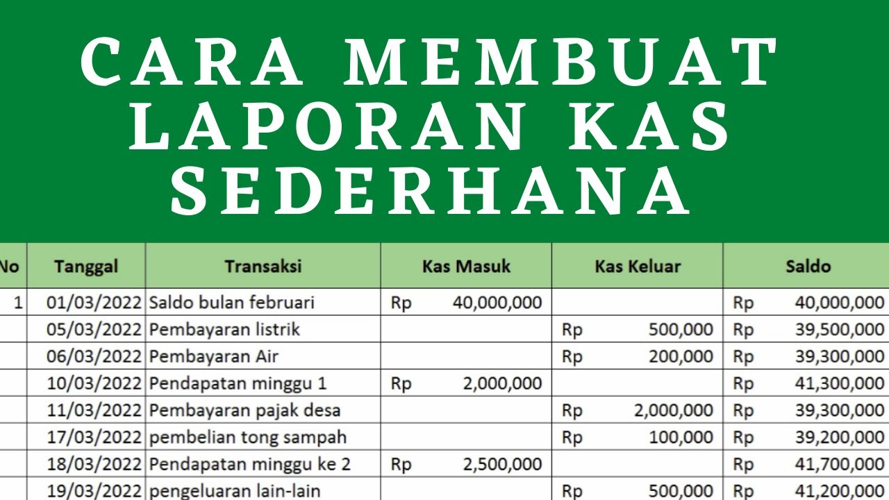
Interactive Excel Dashboard Tutorial in 3 Steps (+ FREE Template)
Cara membuat Laporan Keuangan di Excel dengan Cepat
How to create your own Habit Tracker in Google Sheets - TUTORIAL + FREE TEMPLATE
Excel Tutorial for Beginners
Excel Tutorial for Beginners | Excel Made Easy
5.0 / 5 (0 votes)