Calculus - Average rate of change of a function
Summary
TLDRThis video script delves into the concept of the average rate of change of a function, a fundamental topic in calculus. It explains two methods to calculate this rate: one that requires knowing the exact coordinates of two points on the function, and another, the difference quotient, which simplifies the process by using a single point and the distance from it. The script emphasizes the practicality of the difference quotient for computing average rates of change, especially when dealing with limits, and promises further examples in upcoming videos.
Takeaways
- 📚 The average rate of change of a function is a measure of how much the output (y-values) changes relative to the input (x-values) between two points.
- 📈 There are multiple methods to calculate the average rate of change, but the script focuses on two primary approaches: graphical and analytical.
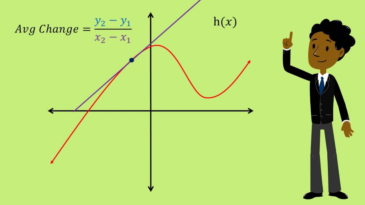
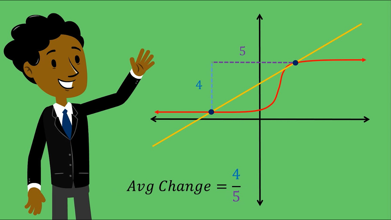
- 🔍 The graphical approach involves drawing a secant line between two points on the graph of a function and calculating its slope.
- 📍 To find the slope of the secant line, one must identify the x and y values of two points, labeled as (X1, f(X1)) and (X2, f(X2)).
- 🧭 The formula for the slope of the secant line is given by (f(X2) - f(X1)) / (X2 - X1), which represents the average rate of change between the two points.
- 🔄 An alternative analytical method defines the second point in terms of a distance 'h' from the first point, with coordinates (X1 + h, f(X1 + h)).
- 📝 The difference quotient is introduced as a formula to compute the average rate of change using the first point and a distance h: (f(X1 + h) - f(X1)) / h.
- 🔑 The difference quotient is advantageous because it only requires knowledge of one point and the distance to the second point, simplifying calculations as the second point moves.
- 📉 As the distance 'h' approaches zero, the difference quotient can be used to find the instantaneous rate of change, which is foundational in understanding limits in calculus.
- 👨🏫 The script suggests that understanding the difference quotient is crucial for deeper study in calculus, particularly when exploring limits and derivatives.
- 🔍 The video script also implies that the difference quotient will be used in further videos to demonstrate how to find the average rate of change for various functions.
Q & A
What is the average rate of change of a function?
-The average rate of change of a function is a measure of how much the y-values of the function change relative to the change in the x-values between two specific points on the function.
How is the average rate of change of a function typically found?
-The average rate of change is found by calculating the slope of the secant line that passes through two points on the function, which is the difference in y-values divided by the difference in x-values.
What are the two methods mentioned in the script for calculating the average rate of change?
-The two methods mentioned are calculating the slope of the secant line using the coordinates of two points and using the difference quotient, which involves a single point and a distance from that point.
Why is the difference quotient considered a better starting point for computing the average rate of change?
-The difference quotient is considered better because it only requires knowledge of a single point and a distance from that point, making it easier to work with as the second point's location changes.
What is the formula for the difference quotient?
-The difference quotient formula is (f(X1 + H) - f(X1)) / H, where X1 is the x-value of the fixed point and H is the distance from that point.
How does the script suggest defining the second point in the difference quotient method?
-The script suggests defining the second point in terms of a distance H away from the first point, with an x-value of X1 + H.
What is the significance of the secant line in the context of the average rate of change?
-The secant line represents the average rate of change between two points on the function, as its slope is the measure of how the function changes over the interval between those points.
How does the script illustrate the process of finding the average rate of change graphically?
-The script uses a graphical representation of a function with two points marked by blue dots, and it shows the secant line between these points to visually represent the average rate of change.
What is the main advantage of using the difference quotient over the direct method of using two points?
-The main advantage is that the difference quotient simplifies the process when one point is fixed and the other point's location is varied, as it only requires the distance from the fixed point rather than exact coordinates.
Why might knowing the exact coordinates of the second point become impractical in certain situations?
-Knowing the exact coordinates becomes impractical when one point is fixed and the other point's location is continuously varied, as it becomes increasingly difficult to determine the x and y values for the moving point.
How does the script relate the concept of the average rate of change to the study of limits in calculus?
-The script hints that the difference quotient is foundational to understanding limits, suggesting that as the distance H approaches zero, the difference quotient can be used to find the instantaneous rate of change, which is related to derivatives and limits.
Outlines

This section is available to paid users only. Please upgrade to access this part.
Upgrade NowMindmap

This section is available to paid users only. Please upgrade to access this part.
Upgrade NowKeywords

This section is available to paid users only. Please upgrade to access this part.
Upgrade NowHighlights

This section is available to paid users only. Please upgrade to access this part.
Upgrade NowTranscripts

This section is available to paid users only. Please upgrade to access this part.
Upgrade NowBrowse More Related Video
Calculus - Approximating the instantaneous Rate of Change of a Function
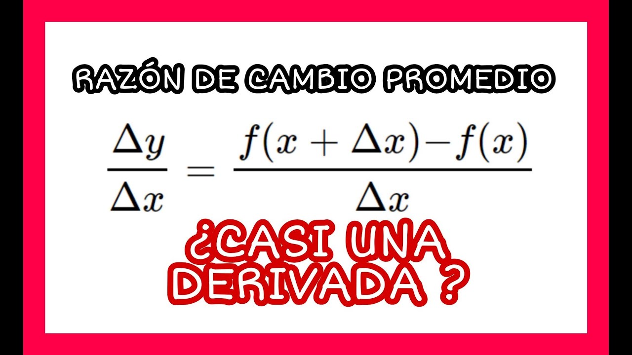
RAZON DE CAMBIO PROMEDIO DE UNA FUNCION. Explicación Detallada Paso a Paso
Calculus - Average Rate of Change of a Function
Average vs Instantaneous Rates of Change

Calculus AB/BC – 2.1 Defining Average and Instantaneous Rate of Change at a Point

What is average rate of change?
5.0 / 5 (0 votes)