Calculus - Average Rate of Change of a Function

Summary

This video script introduces the concept of function behavior in calculus, focusing on how functions increase and decrease. It uses the analogy of a roller coaster to visualize changes and contrasts the steepness of lines to represent different rates of increase. The script explains the importance of slope in describing a function's average rate of change between two points, and hints at the upcoming introduction of limits and instantaneous rates of change as key tools in calculus for a deeper understanding of function behavior.

Takeaways

• 📚 In Calculus, the focus is on understanding how functions change over their domain.
• 🎢 The function's behavior can be visualized as a roller coaster, indicating where it increases and decreases.
• 📈 The concept of a function's increase or decrease is intuitive but requires a precise measure for advanced analysis.
• 📊 Comparing the steepness of functions helps in understanding their rate of increase, which is not immediately intuitive.
• 📐 The notion of slope from linear equations is used to describe the rate of change in the y-direction relative to the x-direction.
• 🔍 The slope of a line can indicate whether one function increases more rapidly than another by comparing their slopes.
• 🤔 For non-linear functions, the idea of slope is adapted by drawing a line (tangent) between two points to approximate the function's change.
• 📉 The slope of such a line represents the average rate of change of the function between the two selected points.
• 🔄 Choosing different points on the function will yield different slopes, thus different average rates of change.
• 🚗 The average rate of change can have real-world applications, such as calculating average speed or flow rates.
• 🔮 The script introduces the concept of limits as a major tool in calculus for finding the instantaneous rate of change of a function at a single point.

Q & A

What is the main focus of the video script in terms of functions?

The main focus is on understanding how functions change and the concept of their rates of increase or decrease.

How does the script suggest visualizing the changes in a function?

The script suggests visualizing a function as a roller coaster to easily see where it increases and decreases.

What is the problem with just knowing if a function increases or decreases?

While knowing if a function increases or decreases tells us about its behavior, it is not precise enough for detailed analysis and comparison of different functions.

How does the script compare the steepness of two increasing functions?

The script compares the steepness by observing the slope of the lines representing the functions, with a steeper line indicating a more rapid increase.

What concept from working with lines is used to describe the rate of change of functions?

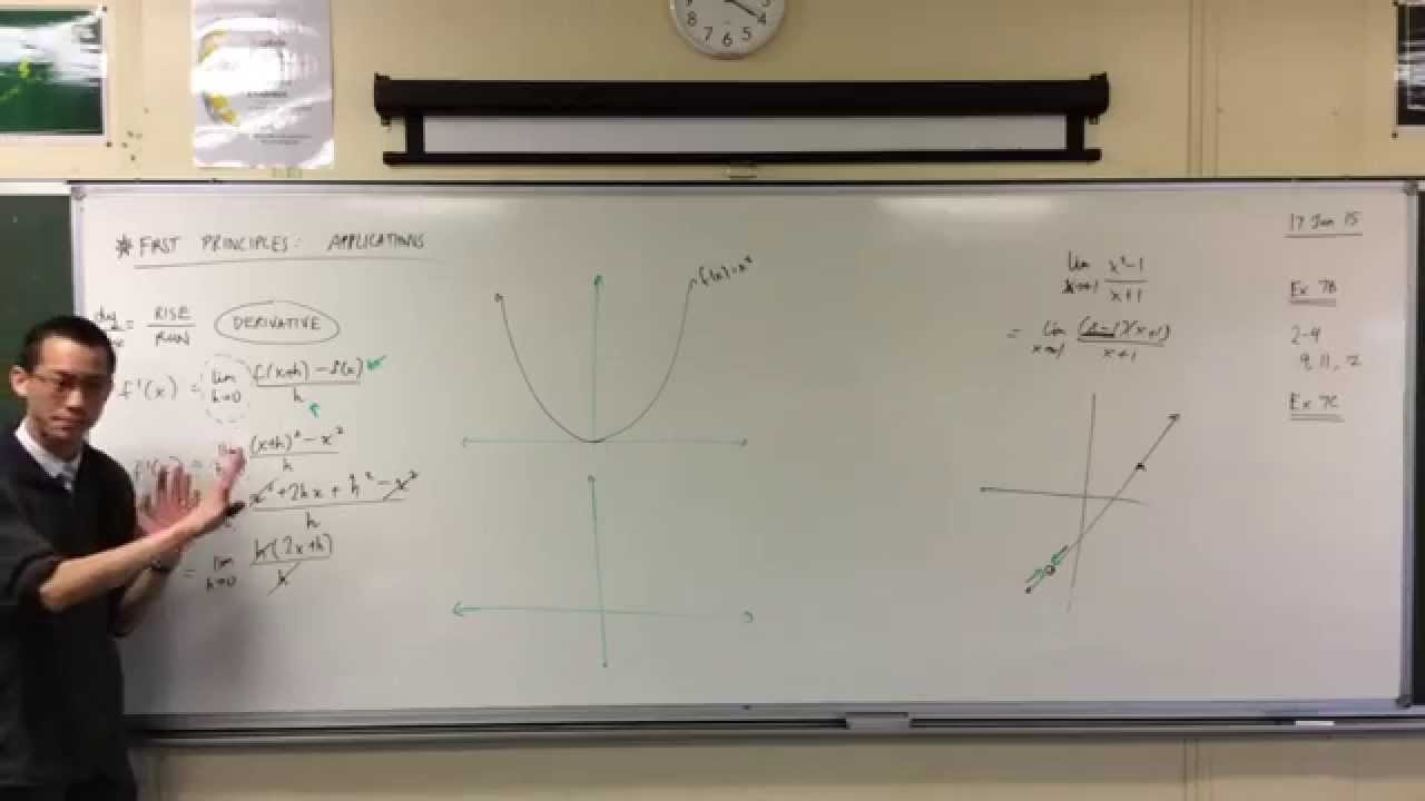
The concept of slope is used to describe the rate of change of functions, by measuring the rise over the run between two points.

Why can't the idea of slope be directly applied to non-linear functions?

The idea of slope cannot be directly applied to non-linear functions because they do not have a constant rate of change like lines do.

How can a line be used to approximate the change of a non-linear function?

By choosing two points on the non-linear function and drawing a line through them, the slope of this line can be used as an approximation of the function's rate of change between those points.

What does the slope of a line between two points on a function represent?

The slope of a line between two points on a function represents the average rate of change of the function between those points.

How does the script use the concept of slope to explain the average change of a function?

The script uses the slope to explain that the average change of a function between two points is the ratio of the change in the y-direction to the change in the x-direction.

What is the next step after understanding the average rate of change?

The next step is to learn how to describe how a function changes at a single point, which will involve the concept of limits and instantaneous rate of change.

What tool of calculus is mentioned as the first major tool to be introduced in the script?

The first major tool of calculus mentioned is the limit, which will be used to describe the function's change at a single point.

Where can viewers find example problems about the average rate of change of a function?

Viewers can find example problems about the average rate of change of a function on the provided website: MySecretMathTutor.com.

Outlines

00:00

📈 Understanding Function Behavior in Calculus

This paragraph introduces the concept of analyzing how functions change in Calculus. It uses the analogy of a roller coaster to describe the increase and decrease of a function's value. The paragraph emphasizes the need for a precise way to measure the rate at which a function increases or decreases, leading to the idea of slope in the context of lines. It sets the stage for the introduction of the limit, which will be used to describe the function's behavior at a single point, rather than between two points.

📉 Comparing Function Growth Using Slope

The second paragraph delves into the comparison of how two functions increase, using the concept of slope to illustrate the difference in their rates of increase. It explains that a steeper function has a larger slope, indicating a more rapid increase. The paragraph also introduces the idea of using the slope of a line to approximate the average rate of change of a function between two points, providing a method to compare the behavior of different functions.

🔍 The Concept of Average Rate of Change

This paragraph explains the concept of the average rate of change by using the slope of a line drawn between two points on a function. It clarifies that this slope represents the average change in the y-direction for a given change in the x-direction. The paragraph provides examples to illustrate how different lines with varying slopes can indicate different average rates of change, and how this can be applied to real-world scenarios such as calculating average speed or flow rate.

🚀 Transitioning to Instantaneous Rate of Change

The final paragraph of the script wraps up the discussion on the average rate of change and introduces the concept of the instantaneous rate of change. It hints at the use of limits to find this rate at a single point, which is a fundamental tool in calculus. The paragraph also invites viewers to explore example problems and further lectures on the topic, and encourages them to visit the tutor's website for more resources.

Keywords

💡Calculus

Calculus is a branch of mathematics that deals with the study of rates of change and accumulation. In the context of the video, it is the central theme as it discusses how to understand and quantify the changes in functions, which is a fundamental concept in calculus.

💡Function

A function in mathematics is a relation between a set of inputs and a set of permissible outputs with the property that each input is related to exactly one output. The video script uses functions to illustrate the concept of change and how calculus helps in understanding the behavior of these changes.

💡Increase and Decrease

These terms describe the behavior of a function as it either gains or loses value. In the video, the instructor uses the idea of a function increasing and decreasing to introduce the concept of the function's rate of change, which is essential for understanding calculus.

💡Roller Coaster

The roller coaster analogy is used in the video to visualize the ups and downs of a function, making it easier to understand where a function increases or decreases. This analogy helps in conceptualizing the changes in the function's value.

💡Steepness

Steepness in the context of the video refers to the rate at which a function increases or decreases. A steeper function indicates a more rapid change, which is a key aspect when comparing the behavior of different functions.

💡Slope

Slope is a measure of the steepness of a line, calculated as the ratio of the vertical change to the horizontal change between two points. In the video, slope is introduced as a way to describe the rate of change for lines, which is later extended to non-linear functions.

💡Average Change

The concept of average change in the video refers to the change in the function's value over an interval, calculated by the slope of the line connecting two points on the function. It provides insight into the general behavior of the function between those points.

💡Approximation

Approximation is used in the video to describe the process of using a straight line (or tangent) to estimate the behavior of a function at a point or over an interval. This is a precursor to the more precise concept of limits and derivatives in calculus.

💡Limit

The limit is a fundamental concept in calculus that describes the value that a function or sequence 'approaches' as the input or index approaches some value. In the video, the limit is mentioned as the next major tool in calculus for describing the function's behavior at a single point.

💡Instantaneous Rate of Change

This term refers to the rate of change of a function at a specific point, as opposed to over an interval. The video script builds up to this concept by first discussing the average rate of change and then indicating that calculus can provide a tool for finding this instantaneous rate.

💡MySecretMathTutor.com

This is the website mentioned in the video for additional resources. It serves as an example of how viewers can seek further information or examples to deepen their understanding of calculus and its applications.

Highlights

In Calculus, the focus is on understanding how functions change over time.

The concept of a function increasing or decreasing is intuitive and can be visualized like a roller coaster.

Comparing the rate of increase between two functions requires a precise measure beyond just observation.

The steepness of a function can indicate how rapidly it is increasing, but a more accurate measure is needed.

Slope is used in linear functions to describe the rate of increase or decrease.

The slope is calculated by the ratio of the rise over the run, offering a precise measure of change.

Non-linear functions cannot be directly described by slope, prompting the need for an alternative approach.

By selecting two points on a function, a line can be drawn to approximate the function's change between those points.

The slope of the line through two points on a function represents the average rate of change over that interval.

Different pairs of points can yield different slopes, indicating varying average rates of change.

A horizontal line through two points on a function indicates no average change in the function's value.

The concept of slope can be applied to functions to understand their average behavior between points.

The average rate of change can have practical implications, such as calculating average speed or flow rates.

The video will introduce the concept of the limit as a major tool in calculus for describing changes at a single point.

The video encourages viewers to like, subscribe, and explore more example problems on the provided website.

The next lecture will cover approximating the instantaneous rate of change of a function.

The presenter invites viewers to visit MySecretMathTutor.com for more educational content.

Transcripts

In Calculus we'll be working with many different

types of functions. One of the major things we'll be interested

in is how these functions change. Fortunately this idea is very intuitive and

you may have started to do this already in previous math courses.

Let's take a look at a quick example to see how we do this.

If we read a function from left to right we can see that sometimes it increases, and other

times it decreases. I like to imagine the function as a roller

coaster so that I can easily see places where it is going up, versus where it is going down.

Knowing how a function increases and decreases certainly tells us more about the behaviors

of a function, but it's still not precise enough for what we will need later.

To see why, let's look at two more functions. Here are two function that are both increasing.

But one is increasing more rapidly. After all it looks steeper.

But how steep is it? Where does it increase the most?

From these questions you can see we need some way to describe how rapidly the function is

increasing or decreasing so we can better compare their behavior.

Let's take a step back. If these two function were lines, this would

be a much easier problem. When we are working with lines we can use

the notion of slope to accurately describe how quickly a line is increasing or decreasing.

This comes from measuring the rise of the function in the y direction, versus the run

of the function in the x direction. With slope we can say how much it is increasing

or decreasing by simply giving this ratio of numbers.

So we can say that the line on the right is increasing more, simply because it has a larger

value for its slope.

Now back to our other functions. These function are definitely not lines so

unfortunately we can't use the idea of slope to describe how they are changing... or can

we?

To build a line all we need are two points. If we choose two points on our function then

we can certainly draw a line right through them.

Note how the line works as a good approximation when describing how the function is changing.

If the line we draw is steep, then we can expect that our function is increasing fairly

quickly as well. But it is only an approximation right now.

If we change the two points we are using, we will get a different value for the slope

of the line. What this line really tells us then is the

average change of the function. How much the function has changed in the y-direction

versus the x-direction between the two given points.

Let's play around with this idea so that it makes a bit more sense.

Suppose we choose two points on a function. Drawing our line like earlier, we can find

it has a slope of 2/3. This tells us that as we are moving on the

function between the two points, we may go up, we may go down, but on average we'll increase

in the y-direction by 2 as we move in the x-direction by 3.

Or, maybe a better way to say this is that the average change of the function between

the two points is also 2/3.

If we choose two other points, our line is now horizontal.

This has a slope of zero. If we move along the function now, you'll

notice that despite the ups and downs, we will end up at the other point at the same

y-value. So on average, there is no change in the function.

So by describing the slope of a line between two points on a function we can get a lot

of information about the behavior, specifically it average rate of change.

Depending on what the function describes this could give us information like the average

speed of a car or the average flow rate from a tank of water.

The possibilities are endless.

But that's not all we can do. Next you'll see how we can use this average

rate of change to describe how a function is changing at a single point, rather than

between two points, and along the way we'll pick up our first major tool of calculus,

the limit.

Thanks for watching.

Did you enjoy this video? Don't forget to like it, and then subscribe

to my channel! If you want to see some example problems about

the average rate of change of a function, you can find those here.

You can also skip ahead to the next lecture where I cover approximating the instantaneous

rate of change of a function. Of course I have many more videos that can

be found on my website: MySecretMathTutor.com So don't forget to stop by.

Thanks for watching!