Understanding Sensor Fusion and Tracking, Part 4: Tracking a Single Object With an IMM Filter
Summary
TLDRThis video introduces the concept of tracking remote objects using estimation filters, transitioning from positioning and localization to single object tracking. It explains the challenges of tracking with limited information and introduces the Interacting Multiple Model (IMM) filter. The video compares single model filters to IMMs, demonstrating how IMMs improve state estimation for maneuvering objects by blending predictions from multiple models. It also discusses the prediction and correction process, the importance of sensor fusion, and the computational trade-offs in using multiple models for tracking. The next video will address the complexities of tracking multiple objects.
Takeaways
- 🔍 The video focuses on the shift from self-positioning to tracking a remote object, emphasizing the importance of state estimation in both scenarios.
- 📈 The video introduces the Interacting Multiple Model (IMM) filter as a solution for tracking uncertain objects, highlighting its effectiveness over single model filters.
- 🛠 The IMM filter is explained as an upgrade to single model estimation filters, allowing for better handling of less information and uncertainty in tracking.
- 🎯 The script discusses the challenges of tracking, such as dealing with less information and the potential for false positive results in data association.
- 🤖 The importance of fusing data from multiple sensors to get a comprehensive measurement of the tracked object is emphasized.
- 🔄 The 'predict and correct' process of estimation filters is outlined, explaining how it applies to both self-state estimation and remote object tracking.
- 🚀 The video uses an airplane example to illustrate the prediction problem in tracking, showing the difficulty in predicting the future state of an uncontrolled object.
- 🔄 The concept of process noise is introduced, explaining its role in accounting for uncertainty in predictions and its impact on filter performance.
- 🔄 The difference between cooperative and uncooperative tracking is discussed, with the latter requiring the filter to treat control inputs as unknown disturbances.
- 🤝 The IMM approach is described as running multiple models simultaneously, each representing a different expected motion of the tracked object.
- 🔄 The video explains how the IMM filter interacts by mixing state estimates and covariances of models after measurements, improving the overall estimation quality.
- 🚀 The computational cost and the need for a smart approach to selecting models for the IMM filter are discussed, warning against using too many models which can degrade performance.
Q & A
What is the main focus of the video?
-The video focuses on switching from estimating the state of our own system to estimating the state of a remote object, specifically discussing the concept of single object tracking and the use of an Interacting Multiple Model (IMM) filter for state estimation in uncertain scenarios.
What is the difference between positioning and localization and single object tracking?
-Positioning and localization are about determining the state of one's own system, while single object tracking is about determining the state of a remote object, such as its position or velocity, by fusing sensor data and models.
Why is tracking a remote object more challenging than estimating the state of our own system?
-Tracking a remote object is more challenging because it often requires working with less information and dealing with uncertainties. The lack of direct control over the remote object and the need to rely on external sensors add complexity to the tracking process.
What is an Interacting Multiple Model (IMM) filter and how does it help in tracking?
-An Interacting Multiple Model (IMM) filter is an advanced estimation filter that combines multiple models to predict and estimate the state of a system. It is particularly useful for tracking uncertain objects by blending the results from different models based on their likelihood of representing the true motion.
What is the significance of the example tracking maneuvering targets in the video?
-The example tracking maneuvering targets is used to demonstrate the effectiveness of the IMM filter. It simulates tracking an object that goes through three distinct maneuvers, showing how the IMM filter can adapt and provide better estimation compared to a single model filter.
How does the IMM filter differ from a single model filter in terms of tracking performance?
-The IMM filter provides better tracking performance by using multiple models to account for different possible motions of the tracked object. It can quickly adapt to changes in the object's motion, resulting in lower tracking error compared to a single model filter that may not match the actual motion.
What are the three types of motion that the IMM filter considers when predicting the future state of an object?
-The IMM filter considers three types of motion: 1) Dynamics and kinematics of the system that carry the current state forward, 2) Commanded and known inputs into the system that change the state, and 3) Unknown or random inputs from the environment that affect the state.
What is the role of process noise in the IMM filter?
-Process noise in the IMM filter represents the uncertainty in the prediction. A higher process noise indicates less confidence in the prediction, allowing the filter to rely more on the sensor measurements for correction.
How does the IMM filter handle transitions between different motions of the tracked object?
-The IMM filter allows models to interact after a measurement, reinitializing each filter with a mixed estimate of state and covariance based on their probability of being switched to or mixing with each other. This helps in reducing the transient error and quickly adapting to new motions.
What is the computational cost of using an IMM filter with a large number of models?
-Using an IMM filter with a large number of models increases the computational cost due to the need to run multiple predictions simultaneously. This can be a limitation in real-time tracking applications where processing time is critical.
Why might having too many models in an IMM filter negatively impact its performance?
-Having too many models can lead to increased transitions between models, making it harder to determine when a transition should occur. It can also result in similar motions being represented by multiple models, which can confuse the filter and lead to less optimal estimation.
What is the next step after understanding single object tracking with an IMM filter?
-The next step is to expand the concept to tracking multiple objects simultaneously, which introduces additional complexities and will be covered in a future video.
Outlines

This section is available to paid users only. Please upgrade to access this part.
Upgrade NowMindmap

This section is available to paid users only. Please upgrade to access this part.
Upgrade NowKeywords

This section is available to paid users only. Please upgrade to access this part.
Upgrade NowHighlights

This section is available to paid users only. Please upgrade to access this part.
Upgrade NowTranscripts

This section is available to paid users only. Please upgrade to access this part.
Upgrade NowBrowse More Related Video
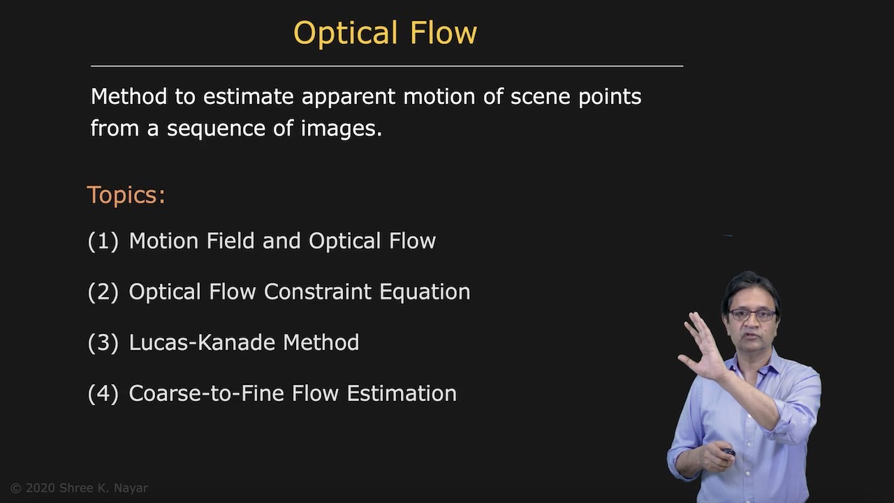
Overview | Optical Flow

Understanding Sensor Fusion and Tracking, Part 3: Fusing a GPS and IMU to Estimate Pose

How To MOTION TRACK Objects In Davinci Resolve

Salesforce Custom Object For B2B Funnel Tracking
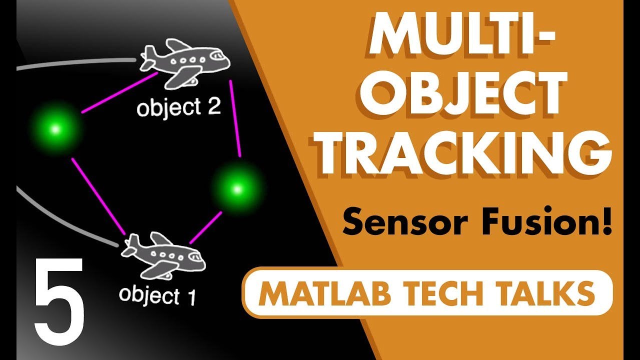
Understanding Sensor Fusion and Tracking, Part 5: How to Track Multiple Objects at Once

SLAM C 01
5.0 / 5 (0 votes)