Least squares comparison with Maximum Likelihood - proof that OLS is BUE
Summary
TLDRIn this video, the presenter compares least squares estimators (LSE) and maximum likelihood estimators (MLE) for linear regression models, demonstrating that LSEs are the best unbiased estimators (BLUE) under certain conditions. By analyzing the second derivative of the log-likelihood function, the presenter shows that the maximum likelihood estimator for the parameter beta has the same estimated variance as LSE, proving that LSE achieves the Cramer-Rao lower bound. This implies that LSEs are the unbiased estimators with the lowest variance, reinforcing their status as BLUE estimators.
Takeaways
- 😀 The video focuses on comparing least squares (LS) estimates with maximum likelihood (ML) estimates in linear regression models.
- 😀 The goal is to prove that least squares estimators are not only the best linear unbiased estimators (BLUE) but also the best unbiased estimators overall under certain assumptions.
- 😀 The process starts with deriving the derivative of the log-likelihood with respect to the parameter beta, a key step in obtaining the asymptotic distribution of ML estimates.
- 😀 To find the asymptotic distribution of ML estimates for linear regression, the information matrix is used, which is symmetric and diagonal with two elements: I_beta_beta and I_sigma_sigma.
- 😀 The two parameters in the model are beta and sigma, but the information matrix for this system will have zero values off the diagonal.
- 😀 The asymptotic variance for ML estimators is found by calculating the inverse of I_beta_beta, which is the second derivative of the log-likelihood with respect to beta.
- 😀 The second derivative of the log-likelihood with respect to beta results in a formula involving the sum of squared x_i values.
- 😀 The CRLB (Cramér-Rao Lower Bound) for the variance of ML estimators is equivalent to the variance obtained through least squares, indicating that both methods yield the same estimated variance for beta.
- 😀 Since least squares estimators achieve the Cramér-Rao Lower Bound, they must be the best unbiased estimators with the lowest variance among all unbiased estimators.
- 😀 The video concludes that least squares estimators, despite being BLUE, also have the lowest variance, which makes them the best unbiased estimators in the given context.
Q & A
What is the focus of the video?
-The video focuses on comparing least squares estimates of linear regression models with maximum likelihood estimates (MLE), and demonstrating that least squares estimators are not only the best linear unbiased estimators (BLUE) but also the best unbiased estimators (BUE).
What are the key assumptions mentioned in the video about least squares estimators?
-The video suggests that least squares estimators are BLUE under certain assumptions, and under additional assumptions, they are proven to be the best unbiased estimators (BUE) as well.
What is the role of the information matrix in the MLE process?
-The information matrix helps in deriving the asymptotic distribution of the maximum likelihood estimates by involving the second derivatives of the log likelihood with respect to the model parameters, in this case, beta and sigma.
How is the information matrix structured for this particular model?
-In this model, the information matrix is symmetric and diagonal, containing two elements: I_beta_beta in the top left and I_sigma_sigma in the bottom right. The other two entries are zero.
How is the second derivative of the log likelihood with respect to beta calculated?
-The second derivative of the log likelihood with respect to beta involves a term of the form (1/sigma^2) multiplied by the sum of x_i^2, where x_i represents the input variable values, leading to the I_beta_beta term in the information matrix.
What is the significance of the inverse of the second derivative term in the MLE process?
-The inverse of the second derivative term gives the asymptotic variance of the maximum likelihood estimator for beta. This step is crucial for determining the variability of the MLE estimates.
How does the CRLB relate to the variance of beta hat in the least squares method?
-The Cramer-Rao Lower Bound (CRLB) represents the lower bound of the variance for any unbiased estimator. In this case, the variance of beta hat from the least squares method is equal to the CRLB, indicating that least squares estimators are the most efficient unbiased estimators.
What does the equality of variance between MLE and least squares estimators suggest?
-The equality of variance between the maximum likelihood estimator (MLE) and the least squares estimator suggests that both estimators are equally efficient in terms of variance, implying that least squares estimators achieve the Cramer-Rao Lower Bound.
Why are least squares estimators considered BLUE?
-Least squares estimators are considered BLUE because, under the right assumptions (such as linearity and normality), they are the best linear unbiased estimators, meaning they have the lowest possible variance among all unbiased linear estimators.
What does it mean that least squares estimators are the best unbiased estimators?
-Being the best unbiased estimators means that least squares estimators not only provide an unbiased estimate of the parameter (beta), but also minimize the variance of that estimate, making them the most efficient among all unbiased estimators.
Outlines

This section is available to paid users only. Please upgrade to access this part.
Upgrade NowMindmap

This section is available to paid users only. Please upgrade to access this part.
Upgrade NowKeywords

This section is available to paid users only. Please upgrade to access this part.
Upgrade NowHighlights

This section is available to paid users only. Please upgrade to access this part.
Upgrade NowTranscripts

This section is available to paid users only. Please upgrade to access this part.
Upgrade NowBrowse More Related Video

Lec-5: Logistic Regression with Simplest & Easiest Example | Machine Learning
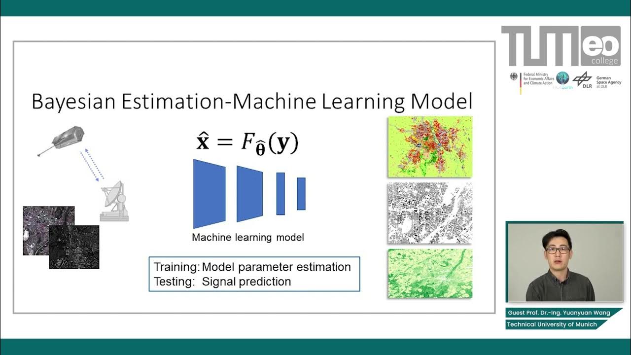
Bayesian Estimation in Machine Learning - Maximum Likelihood and Maximum a Posteriori Estimators

Bayesian Estimation in Machine Learning - Introduction and Examples

Lecture 9.3 _ Parameter estimation: Error in estimation
Regresion Lineal
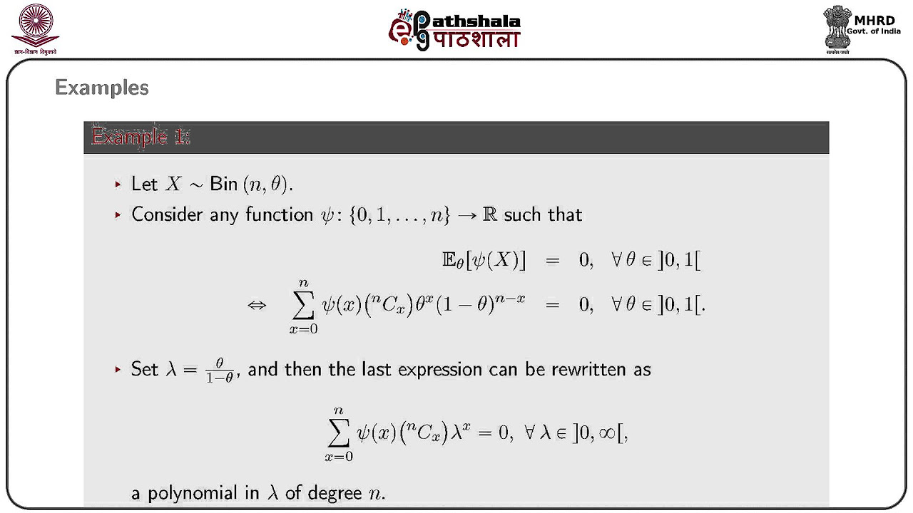
Completeness
5.0 / 5 (0 votes)