13.2 Fonctions du 1er degré , racine et ordonnée à l'origine
Summary
TLDRThis video script explains the core concepts of first-degree functions, including affine, linear, and constant functions. It covers how to determine the root and ordinate at the origin for each function type, with practical examples. The affine function is shown to have a root and ordinate at the origin determined by its equation, while the linear function always passes through the origin. Constant functions are parallel to the X-axis and don't have a root. The video also explains graphical representations of these functions, emphasizing the importance of understanding how roots and ordinates impact their graphs.
Takeaways
- 😀 Affine functions are expressed in the form y = MX + P, where M is the slope and P is the y-intercept.
- 😀 The root (or zero) of an affine function is the value of x when y = 0, calculated as x = P / M.
- 😀 The ordinate at the origin of an affine function is always equal to P, the y-intercept.
- 😀 For example, in the affine function y = -2x + 4, the root is x = 2 and the ordinate at the origin is y = 4.
- 😀 Linear functions are a special case of affine functions where the constant term P is zero, making the equation y = MX.
- 😀 The root of a linear function is always x = 0, and the ordinate at the origin is always y = 0.
- 😀 A constant function is a degree 0 function expressed as y = P, where M = 0 and the graph is parallel to the x-axis.
- 😀 Constant functions do not have a root, as their graph never intersects the x-axis, but their ordinate at the origin is always equal to P.
- 😀 A relation like x = N represents a vertical line in the graph, but it is not a function because for a single x-value, there are multiple corresponding y-values.
- 😀 The graphical representation of affine and linear functions is a straight line, with affine functions potentially not passing through the origin, while linear functions always do.
Q & A
What is the general form of an affine function?
-The general form of an affine function is y = MX + P, where M is the slope and P is the y-intercept.
How do you find the root of an affine function?
-The root of an affine function is found by setting y = 0 and solving for x. The root is given by x = -P / M.
What does the root of an affine function represent?
-The root of an affine function represents the value of x where the graph of the function intersects the x-axis, i.e., where y = 0.
What does the y-intercept represent in an affine function?
-The y-intercept in an affine function is the value of y when x = 0. It is represented by the constant P in the function y = MX + P.
How do you determine the root and y-intercept for the function y = -2x + 4?
-For the function y = -2x + 4, the root is calculated as x = -4 / -2 = 2, and the y-intercept is P = 4.
What is the root and y-intercept for the function y = 2x - 1?
-For y = 2x - 1, the root is x = 1/2, and the y-intercept is P = -1.
What is the graphical representation of an affine function?
-The graphical representation of an affine function is a straight line. The slope M determines the steepness, and the y-intercept P determines where the line crosses the y-axis.
How do you calculate values for plotting the graph of an affine function?
-To plot the graph of an affine function, you can create a table of correspondence by selecting different x values and calculating the corresponding y values using the function formula.
What is the difference between an affine function and a linear function?
-The key difference is that in a linear function, the constant term P equals 0, meaning the function passes through the origin (0,0), while an affine function may not.
What is the graphical behavior of constant functions?
-Constant functions, like y = P, produce horizontal lines parallel to the x-axis. These functions have no roots, and their y-intercept is always P.
Outlines

This section is available to paid users only. Please upgrade to access this part.
Upgrade NowMindmap

This section is available to paid users only. Please upgrade to access this part.
Upgrade NowKeywords

This section is available to paid users only. Please upgrade to access this part.
Upgrade NowHighlights

This section is available to paid users only. Please upgrade to access this part.
Upgrade NowTranscripts

This section is available to paid users only. Please upgrade to access this part.
Upgrade NowBrowse More Related Video

ESTUDO DAS FUNÇÕES: FUNÇÃO AFIM - PARTE I ( AULA 3 DE 9 ) | MATEMÁTICA INTEGRAL

FUNÇÃO AFIM - EXERCÍCIOS # 1
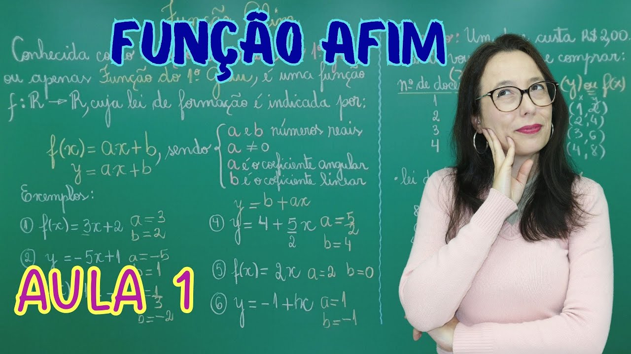
FUNÇÃO AFIM | FUNÇÃO DO 1º GRAU | LEI DE FORMAÇÃO | AULA 1 - Professora Angela Matemática

FUNÇÃO DO 1º GRAU: DEFINIÇÃO E GRÁFICO

FASE 4 - VIDEOAULA 1 - MATEMÁTICA - DESAFIO CRESCER SAEB (3ª SÉRIE)
Illustrate Polynomial Functions | Second Quarter | Grade 10 MELC
5.0 / 5 (0 votes)