Lecture 25 : Binary Search Tree (BST) Sort

Summary

The video script introduces the concept of binary search tree (BST) sorting, explaining how BSTs can be used to create a sorting algorithm. It defines a BST and its properties, contrasting balanced and unbalanced trees. The script then details the BST sort algorithm, which involves inserting elements into a BST and performing an inorder traversal to obtain a sorted sequence. It also discusses the time complexity of building a BST, which can range from O(n log n) in the best case to O(n^2) in the worst case. The script concludes by drawing parallels between BST sort and quicksort, noting their similar time complexities and the number of comparisons involved. The next class will explore the randomized version of BST sort and the expected balanced height of a randomly built BST.

Takeaways

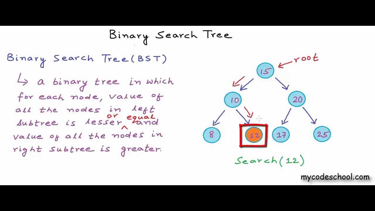
• 🌟 A binary search tree (BST) is a tree data structure where each node has a key value, and all nodes in the left subtree have keys less than the node's key, while all nodes in the right subtree have keys greater than the node's key.
• 📚 BST sort is a sorting algorithm that utilizes the properties of a binary search tree to order elements. It involves inserting elements into a BST and then performing an inorder traversal to retrieve them in sorted order.
• 🔍 The efficiency of a BST depends on its balance. A balanced BST has a height of log n for n nodes, allowing for search and query operations to be performed in logarithmic time.
• 🚀 The process of BST sort involves initializing an empty BST, inserting each element of the array into the BST, and then conducting an inorder traversal of the BST to obtain the sorted elements.
• 🌳 The insertion process in a BST involves starting at the root and moving left or right depending on whether the element to be inserted is less than or greater than the current node's key, continuing until a null position is found where the new element is inserted.
• 📉 The time complexity for an inorder tree walk, which is used to extract the sorted elements from the BST, is O(n), as each node is visited exactly once.
• ⏳ The time complexity to build the BST depends on the nature of the input data. In the best case, with a balanced tree, it is O(n log n), while in the worst case, with an unbalanced tree, it can be O(n^2).
• 🔄 The lower bound for building a BST is O(n log n) because even in the best-case scenario with a balanced tree, each insertion requires a number of comparisons proportional to the height of the tree.
• 🔢 The worst-case scenario for building a BST occurs when the input data is already sorted or reverse sorted, leading to a degenerate tree structure where each insertion requires a comparison with all previously inserted elements.
• 🔗 There is a relationship between the performance of BST sort and quicksort. Both algorithms have the same time complexity in their best and worst cases, and they perform the same number of comparisons when using a stable partitioning method.
• 🎲 The next topic to be discussed is the randomized version of BST sort, which is expected to have a balanced tree height of log n on average, making it more efficient for sorting.

Q & A

What is a binary search tree (BST)?

A binary search tree (BST) is a tree data structure with the property that for any given node with a key value X, all nodes in the left subtree have key values less than X, and all nodes in the right subtree have key values greater than X.

What are the characteristics of a balanced BST?

A balanced BST is one where the height of the tree is log(n), meaning that it maintains a relatively equal distribution of nodes across its levels, ensuring efficient search and insertion operations.

What is the difference between a good and a bad binary search tree?

A good binary search tree is balanced, where the height is log(n). A bad binary search tree is unbalanced, where the height can be as large as n, leading to inefficient operations.

Why is a balanced BST preferred?

A balanced BST is preferred because it allows for efficient search, insertion, and deletion operations, all of which can be performed in O(log n) time, as opposed to O(n) in an unbalanced tree.

What is BST sort?

BST sort is a sorting algorithm that involves inserting elements into a BST and then performing an inorder traversal to retrieve the elements in sorted order.

How does the BST insert operation work?

The BST insert operation starts with the root and compares the value to be inserted with the current node's value. If the value is less, it moves to the left subtree; if greater, to the right subtree, continuing this process until it finds an appropriate position to insert the new node.

What is an inorder traversal in a BST?

An inorder traversal in a BST involves visiting the left subtree, then the root node, and finally the right subtree. This traversal method retrieves the elements in sorted order.

What is the time complexity of inorder traversal in a BST?

The time complexity of inorder traversal in a BST is O(n), where n is the number of nodes, since each node is visited exactly once.

What is the time complexity of building a BST?

The time complexity of building a BST depends on the order of insertion: it is O(n log n) for a balanced tree and O(n^2) for a completely unbalanced tree.

How does the time complexity of BST sort compare to quicksort?

Both BST sort and quicksort have a worst-case time complexity of O(n^2) and a best-case time complexity of O(n log n). The similarity in time complexity arises because both algorithms perform a similar number of comparisons.

Outlines

00:00

🌟 Introduction to Binary Search Tree (BST) Sorting

This paragraph introduces the concept of using binary search trees (BST) for sorting algorithms. It explains what a BST is, highlighting its properties where for any given node with key value X, all left subtree nodes have keys less than X and all right subtree nodes have keys greater than X. The importance of balanced trees is emphasized, with balanced BSTs having a height of log n, which is crucial for efficient search and query operations. The paragraph also outlines the process of BST sorting, starting with an empty BST and inserting elements from an array into the tree. The final step involves an inorder traversal of the BST to yield a sorted sequence of the input numbers.

05:01

📚 In-Depth Explanation of BST Insertion and Traversal

This section delves into the specifics of BST insertion and traversal. It describes the BST insertion process, where a new node is placed in the correct position within the tree by comparing it with existing nodes, moving left or right as necessary. The paragraph also explains the inorder tree traversal method, which visits all nodes in a sorted order by traversing the left subtree, then the root, and finally the right subtree. An example is given to illustrate how numbers are inserted into the BST and how the inorder traversal results in a sorted array. The process of BST insertion through recursive calls and the conditions for moving left or right in the tree are also detailed.

10:07

🕵️‍♂️ Analyzing the Time Complexity of BST Sorting

The focus of this paragraph is on analyzing the time complexity of building a BST and performing an inorder traversal. It discusses the lower and upper bounds of the time it takes to build a BST, emphasizing that the time complexity is dependent on the depth of each node in the tree. The lower bound is established as Omega(n log n), indicating that the best-case scenario involves a balanced tree where each insertion requires log n comparisons. The upper bound is explored in the context of a 'bad' tree, which could result in a time complexity of O(n^2) if the tree is unbalanced, resembling a linked list. The paragraph concludes by highlighting that the time complexity for BST sort is O(n) for the inorder traversal plus the time taken to build the BST.

15:11

🔄 Comparing BST Sort with Quick Sort Time Complexities

This paragraph compares the time complexities of BST sort and quick sort, noting that both algorithms share similar performance characteristics. It points out that the worst-case time complexity for BST sort is O(n^2), which occurs when the input data results in an unbalanced tree. Conversely, the best-case scenario for BST sort is O(n log n), assuming a balanced tree. The paragraph also discusses the relationship between the number of comparisons made during a quick sort partition and those made when building a BST, suggesting that the same number of comparisons underlies both algorithms, leading to their similar time complexities. It concludes by drawing a parallel between BST sort and quick sort, both being comparison-based sorts with lower bounds greater than O(n log n).

20:18

🌲 Relationship Between BST Sort and Quick Sort

The paragraph explores the relationship between BST sort and quick sort, demonstrating that the number of comparisons made during the partitioning process of quick sort is equivalent to those made when inserting elements into a BST. Using a specific example, it shows that the same elements are compared in the same order in both algorithms, leading to the same time complexity. The discussion also touches on the concept of a stable partition, which maintains the order of elements within the same partition, and its implications for the comparison process. The paragraph concludes with the observation that the similarity in the number of comparisons explains the identical time complexities for both BST sort and quick sort.

25:18

🎲 Upcoming Discussion on Randomized BST Sort

In this concluding paragraph, the speaker previews the next topic of discussion, which is the randomized version of BST sort. It mentions that the expected height of a randomly built BST will be balanced at log n, indicating a more efficient sorting process. The speaker expresses intent to cover this topic in the next class, providing a segue into further exploration of BST sorting algorithms and their efficiency under different conditions.

Keywords

💡Binary Search Tree (BST)

A binary search tree (BST) is a binary tree data structure where each node has at most two children, referred to as the left child and the right child. The key concept in a BST is that for any given node, all elements in its left subtree are less than the node's key value, and all elements in its right subtree are greater. This property is crucial for the sorting algorithm discussed in the video, as it allows for efficient searching, insertion, and sorting operations. In the script, BST is used to demonstrate how a given array of numbers can be sorted by utilizing the inherent ordering properties of the tree structure.

💡Sorting Algorithm

A sorting algorithm is a method for rearranging a list of items into a particular order, typically ascending or descending. In the context of the video, the binary search tree is used as a sorting algorithm, where the insertion of elements into the BST and subsequent in-order traversal of the tree results in a sorted list. The video script explains how BST sort operates, comparing it to other sorting algorithms like quicksort in terms of time complexity.

💡In-Order Traversal

In-order traversal is a tree traversal method where the left subtree is visited first, then the node itself, and finally the right subtree. This method is significant in the video's discussion of BST sort because performing an in-order traversal on a BST results in the elements being printed in sorted order. The script illustrates this by showing how an in-order traversal of the BST formed from a given array yields a sorted sequence.

💡Balanced Tree

A balanced tree is a binary tree in which the depth of the two subtrees of every node never differs by more than one. This balance is important for maintaining the efficiency of operations like search, insertion, and deletion. In the video, the concept of a balanced tree is used to explain why a BST with a height of log n is considered 'good' because it allows for operations to be performed in O(log n) time, as opposed to a 'bad' tree where the height is n, leading to less efficient operations.

💡Insertion

Insertion in the context of a BST refers to the process of adding a new element to the tree while maintaining the BST properties. The video script describes the BST insert operation, where a new node is placed in the correct location to ensure that the left subtree contains only elements less than the node's key and the right subtree contains only elements greater. This process is fundamental to the BST sort algorithm, as it builds the initial tree structure from the unsorted array.

💡Time Complexity

Time complexity in computer science is a measure of how long an algorithm takes in terms of the amount of input. The video script analyzes the time complexity of the BST sort algorithm, discussing its lower and upper bounds. It explains that the time to build a BST is dependent on the depth of the nodes and that the best-case scenario (a balanced tree) has a time complexity of O(n log n), while the worst-case scenario (an unbalanced tree) has a time complexity of O(n^2).

💡Quick Sort

Quick sort is a comparison-based sorting algorithm that works by selecting a 'pivot' element from the array and partitioning the other elements into two sub-arrays, according to whether they are less than or greater than the pivot. The script draws a parallel between the time complexity of quick sort and BST sort, noting that both have a worst-case time complexity of O(n^2) and a best-case time complexity of O(n log n). It also suggests a relationship between the number of comparisons made during the partitioning of quick sort and the insertions in BST sort.

💡Stable Partition

A stable partition, as mentioned in the context of quick sort in the video, is a partitioning of an array where the relative order of elements within the same partition is maintained. The script discusses the difficulty of achieving a stable partition and its importance in ensuring that the number of comparisons made during the quick sort partitioning is equivalent to those made when building a BST, thus explaining the similar time complexities of both algorithms.

💡Worst-Case Scenario

The worst-case scenario refers to the situation where an algorithm takes the maximum possible time to complete, given the worst possible input. In the video, it is explained that for BST sort, the worst-case scenario occurs when the tree is unbalanced, leading to a time complexity of O(n^2). This happens when the input array is already sorted or reverse sorted, resulting in a tree that is essentially a linked list.

💡Best-Case Scenario

The best-case scenario is the opposite of the worst-case scenario, where an algorithm performs optimally given the most favorable input. The video script explains that for BST sort, the best-case scenario is when the tree is perfectly balanced, which results in a time complexity of O(n log n). This is because each insertion requires a logarithmic number of comparisons, making it the most efficient situation for the algorithm.

Highlights

Binary search tree (BST) is a tree data structure with specific ordering properties.

BST nodes have left subtree with smaller keys and right subtree with larger keys.

Balanced BSTs are preferred for efficient search operations, with height proportional to log n.

BST sort is a sorting algorithm that utilizes the properties of BSTs.

BST sort involves inserting elements into an initially empty BST.

Inorder traversal of a BST results in a sorted sequence of elements.

The process of BST insertion is detailed, including handling of leaf nodes.

An example is given to illustrate the formation of a BST and subsequent inorder traversal.

Time complexity of inorder tree walk is O(n), as each node is visited once.

The time to build a BST depends on the depth of each node and can vary.

Lower bound for building a BST is Ω(n log n), assuming a balanced tree.

Upper bound for the worst case of building a BST is O(n^2) for an unbalanced tree.

BST sort's time complexity is compared to quicksort, sharing similar bounds.

The relationship between BST sort and quicksort is explored, noting similar comparison counts.

Quicksort's partitioning process is analogous to BST insertion in terms of comparisons.

The concept of stable partition in quicksort is introduced.

Randomized version of BST sort and expected height of randomly built BSTs will be discussed in the next class.

BST sort and quicksort both being comparison-based sorts have a lower bound of Ω(n log n).

Transcripts

An Introduction to Algorithms

So we talk about binary search tree sorting I mean how binary search tree can help us

to have a sorting algorithm. So, before that let us talk about what is the binary, recap

the binary search tree, binary search tree or in sort it is call BST.

So, it is basically a tree and it has some property when it is search property. What

is that? It is suppose we take, so this is a tree suppose you take any node over here

in this tree this is key value is X. Now we considered the left subtree rooted at this

right subtree rooted at this. Now binary search tree means all the key value over here must

be less than X all the value must be greater than X. So, this is the property. So, if they

distinct then it is must be strictly this. So, this is the property of binary search.

So, a binary tree which is having this property is called binary search tree. So, if the all

elements in the left side of the tree is less than X and all the element in the right side

of the tree must be greater than X. So, there are some good tree and bad tree. So, what

are the good tree? So, suppose we have a tree like this, this is a good binary tree why

because it is balanced this one is good tree, good in the sense it is balanced height is

log n. So, if there are n nodes height is log n. So, this is a balanced tree. And what

is the bad tree? Bad binary tree like this if we have this. So, say height is n ok. So,

this is a bad tree because it is not balance tree.

So, why balance tree is good because we can do some search or we can do some query in

a height time and if height is log n then it is a log n time. So, that is why if it

is good to have a balance tree. So, today now we will talk about yeah. So, BST sort

binary search tree sort how we can use the binary tree to have a sorting algorithm. So,

let us just talk write this as BST sort. So, we have given n numbers we can sort them by

using the binary search tree.

So, this is BST sort we have given n numbers or we have given a array of size n. So, what

we do? First our t is empty we are initialising a t tree binary search tree empty and then

we will from the tree. So, we just for i is equal to one to n we insert this node into

the tree. So, this is BST insert basically we insert

this A i into the tree and then we will do the inorder traversal of the tree. So, this

is this is after this we form the tree, form the BST. So, we will talk about how the BST

insert will work we form the BST and then so to from BST basically we start with the

root until we reach to a nil or the leaf node, if tree is initially empty then the first

node will be the root and in the subsequence step. So, if we start with the root if the

element is less than that we go to the left side of the root left subtree otherwise we

go to the right subtree and this way you continue until we reach to a nil or leaf node once

we reach to a nil we insert that node there. So, this is the basically BST insert.

And then we do the inorder tree walk inorder tree walk of this tree inorder tree walk means

we first print the this is basically the way to print a tree or a traversal, tree traversal.

So, we first print the leaf subtree then the root then the right subtree. So, that way

we just visit the all the element of the tree. So, this is one. So, there are inorder, pre

order, post order. So, this is the way. So, inorder, if you do

the inorder traversal then we will get the sorted one. So, let us take an example -

suppose we have some number say 3 1 8 2 6 7 5 suppose this is our a array this is our

given numbers, there are how many numbers 1 2 3 4 5 6 7, there are 7 numbers is given.

So, now, how to form the tree? So, initially tree is empty now we insert this 3, 3 will

be the root and then we then we insert slowly, so 1. So, this we have to insert 1. So, we

start with the root 1 is less than 3. So, we will go to the left part of the tree left

part is empty. So, you will insert there 8, 8 is greater than 3, then 2 we start with

the root 2 is less than 3. So, we will go to the left part of the tree

then again 2 is greater than one. So, we will put it here and then 6, 6 is greater than

3, but less than 8. So, we will put it here then 7, 7 is greater than 3, but less than

8 again greater than. So, we will put it here then 5 5 is greater than 8 say greater than

3, but less than 8, but again less than this. So, this is the structure of the tree. So,

basically this is the BST insert. So, BST insert means, if you just write the

BST insert code, BST insert, so we first. So, we first go we first start with the root.

So, we take this X as a root, root of the tree initially root is empty root is null.

So, while we are not reaching to a null while X is not null. So, we do this if the key of

key of X; that means, key key means here the values if the key of x. So, we are going to

insert some number A i, if key of X is less than A i then we call the this is the recursive

call. Then we go to the, then X is this is while loop then X is left of X else X will

be the right of X, if key is greater than this. Ao that means, we start with the root

if the root is empty that is the initial condition t is empty then we insert that that is why

3 is inserted has a root and after that we start with we say 8.

So, we know 8 is greater than this. So, we call this in this then again 8 is sitting

here. So, like this. So, this is the BST insert now what is the inorder tree walk inorder

tree walk basically. So, inorder tree walk. So, inorder tree walk is basically we first,

so X is the root, root of t. So, we first print the we first traverse the left part

of the left of a X then we print the root and then we print the right of X print means

we again call the inorder tree walk. So, we do until we go until it search no child then

we will print it print right of X print means this is basically inorder tree walk again.

So, for example, here we start with we want to call. So, this is our tree after this is

insert BST tree insert. So, we start with the root we first call this inorder tree walk

of this and then we print 3 and then we call the we print the right part of the tree this

is the right part. So, again for the left part so this is the tree now, now we again

call the inorder. So, this has no left part, this is one then we print the right part.

And similarly for this tree, so 8 is the root for this subtree now we call the inorder tree

walk, it will 8 will be. So, there is no right subtree, so 8 will be printed here and this

as to be print the left subtree. So, left subtree is this one. So, again for this we

call this is the root this is the right sub right and this is the left. So, 5 6 7 sorted.

So, inorder tree walk if we if we do the inorder tree of on this BST we are getting the sorted

array. So, this called BST sort. So, now, we have to analysis this how much time it

is taking. So, how much time it is taking how much time it is taking to do this inorder

tree walk it is order of n because basically we are just seeing the node only once we are

just print we are just travelling the tree. So, we are visiting the nodes only once. So,

there are n nodes. So, it is basically order of n we are just printing the nodes. So, order

of n. Now the question is how much time it will

take to build the tree build the BST this is the build the BST. So, how much time it

will take, so time to build the BST, so that is the question. So, that time will depend

on this the total time for the BST sort. So, how much time it will take to build a binary

search tree for a given n input for a given n array. So, how much time it will take to

build a BST? So, we will come back to this example again.

So, time to build BST binary search tree. So, any answer I mean. So, any lower bound

upper bound. So, any upper bound how much time it will take. So, how to build a BST?

So, basically time to build a BST is basically summation of the depth of X, while X in the

tree because. So, we are every time are we are comparing and we are reaching to a position

and that position is the depth of that node. So, depth means that many times we compared

to insert this node. So, this the time complexity to build the BST basically time of the depth

of X where X is in the tree. So, this will be basically big omega of n

log n this is the lower bound we cannot do better than big omega of n log n why because

when is the best case for this when the we have a balance tree if the tree it dependence

on the nature of the tree. If the tree is balanced if the tree is balance suppose there

are n node this is the balance tree if the tree is balance now how much time it will

take to insert how much time it will take to build such a tree. So, how many node are

there here in the leafs? So there are basically n by 2 nodes there are total n nodes and this

is the height, height is basically n height is basically log n base 2. Now this is the

depth of this node this depth is log n. So, for each of this leaf node we have to compare

root then these then these with these then only it came here. So, that is the depth of

this node, depth of this node is log n. So, at least for each of this node we have

to compare log n time. So, n by 2 is log n by 2 n is the comparison for all these node

and even we have these node. So, that is why height is height must. So, time is must be

greater than n log n. So, this is the depth, this must be greater than n log n because

there are n by 2 nodes. So, at least for this node we have to we have to the depth is log

n for this node. So, depth is log n means they have to compare with this node this node.

So, how many comparison at least log n comparison each of this leaf at to compare with the log

n many nodes. So, that is why we inserted in that height level. So, that is why this

time is basically big omega of n log n this is the lower bound. We cannot do better than

this. And any upper bound whether this is any big O. So, this we have to think. So,

this is the best case.

Now can we say this is n square big O of n square. So, when is the worst case of this

scenario? Worst case is if the tree is bad tree like if the tree is like this if there

are n nodes then height. So, then what is the summation of depth of X? X is in tree,

so this basically arithmetic series, so this is n into n plus 1 by 2. So, this is order

of n square. So, if the tree is bad tree so that means, if our numbers search is ascending

order or descending order suppose we have given numbers are like this say 2 4 6 7 8

9 suppose this is our input. Suppose this is our input sorted, the our array is sorted

already then what is the tree, tree will be like this. So, 2 then 4 6 7 8 9 see. So, this

is basically to from this tree we need order of n square because everybody has to compare

with the that previous all the element. Even if it is reverse sorted also this will

be like this if it is reward sorted the tree will be looks like this. So, this is the worst

case. So, worst case is order of n square to build the tree. So, this is the time complexity

for time, time to build the tree. So, this is the worst case so that means so this will

the time for BST sort. So, this will be the time for BST sort because inorder traversal

will take linear time and this will take the measure time will take by here to build BST

to build the binary search tree and that itself is a its taking the time of order of n square.

So, the time complexity for BST sort in the worst case it is order n square and in the

best case it is order of n log n.

So, the time for runtime or time complexity of BST sort. So, worst case it is order of

n square and the best case it is n log n. So, BST sort, this is the sorting algorithm

which is taking worst case what about n square and best case n log n. So, is it remind us

some sorting algorithm we know who performance is like this, like worst case is n square

and the best case is n log n sorry n log n. So, we know any sorting algorithm we have

studied comparison best sort because here this is also the BST sort is also comparison

based sort because this is also a comparison best sort and that is why lower bound has

to more than n log n I mean that is I mean we cannot do better than n log n we have seen

by the this is entry method module that we have seen any comparison best sort worst case

time complexity is more than cannot be faster than the n log n.

So, this is also comparison based sort because we are comparing the element and then we are

forming tree and then we are inorder traversal. So, any comparison based sort we know having

this time complexity yes quick sort. So, quick sort is having same type of time complexity

worst case quick sort worst case is order of n square and the best case is order of

n log n. So, quick sort is having the same time complexity has BST sort. So, that is

the, that is the our next point to see whether is there any relationship between BST sort

and the quick sort why they are giving us the same time complexity. So, that we want

to see that what is the relationship between BST sort and the quick sort. To see that let

us take the example again and we will see that they were having same number of comparison

we are doing in quick sort and the BST sort. So, let us take that same example A array,

8 sorry 3 1 8 2 6 7 5 this is our given input and in the BST sort we form the tree 3 then

1 then 8 then here 2 here 6 and then 5 7.

So, this is the BST binary search tree and then we do the inorder traversal to have this

thing. So, have the sorted one to have the sorted one array. So, this is BST sort. Now

let us talk about quick sort performance on this input. So, in the quick sort what we

are doing we are choosing a pivot element suppose we choose and we choose the first

element as a pivot if we choose the first element as a pivot. So, what will be look

likes 3 is a pivot. So, what pivot will do, pivot will partition this array into 2 sub

array all the element less than X must be left sub array all the element greater than

X possible right sub array. So, that way it will do like this. So, 3 this is the array

3 1 8. So, let us just 3 1 8 2 6 7 5. So, this is the given input now we choose this

as a pivot element. So, it will partition this into two part all

the element will be less than X must be in the left sub array all the element greater

than X must be in the right sub array. So, who are the element? So, 1 2 must be sitting

here and 8 6 7 5. So, this is quick sort partition and here we are assuming one thing this partition

must be stable partition because we are assuming this ordering will not changing. So, we know

this is 1 2 will come in left sub array, but it is not guaranteed that 2 will come. So,

which ordering, but here we are using a partition which is call stable partition and that is

what very tough to get the code of stable partition. So, stable partition means we are

assuming the ordering of this input ordering same has this in the array. So, there are

8 6 7 5 there in the same order. Now again for this we are taking this as a

pivot now all the elements. So, 2 will be sitting here and we are taking this as a pivot.

So, who are element are greater than all the element are greater than less than 8. So,

6 7 5 then 2 then nobody is there then we call 6 is here, so this is basically 5 and

7. So, this is the recursive call of the partition. Now if you just form the tree like this, like

this, so like this if you look this 2 tree as same, so that means, we are doing the same

number of comparison. So, in the partition recursive call of partition the number of

comparison we are doing is same as to form the BST because to form the BST this 6. So,

when you insert 6, 6 as to compare with 3 6 as to compare with 8 here also.

So, to come here 6 as to compare with 3 because this will partitioning into 2 part again 6

as to compare with this 8. So, the same number of comparison we are doing for the both the

cases. So, this is the idea. So, BST sort. So, this is the observation BST sort basically

to form the BST performs the same number of may be different order, but

we are doing same number of comparison as in quick sort same comparison, comparison

as quick sort. So, that is the reason there are giving the same time complexity, the time

complexity is coming out to be same because of this fact that we are basically doing the

same number of comparison in both the cases to form the BST and for the quick sort.

Here we are assuming this stable the partition is stable partition because to and that is

also not tough to achieve to have this 2. So, the same tree we are having this. So,

this is the observation and that is the reason it is giving us the same time complexity for

the BST sort and the quick sort. So, in the next class we will talk about randomized

version of the BST sort and there we will see the height of the randomly build BST.

So, that will expected height we will see to be balanced log n. So, that will cover

in the next class. Thank you.