PENYELESAIAN PDP DENGAN PEMISAHAN VARIABEL BAG 2
Summary
TLDRThis video covers the second step in solving Partial Differential Equations (PDEs) using the method of separation of variables. The focus is on applying boundary conditions, particularly conditions 2A and 2B, which set the function values to zero at both ends of the domain. The discussion includes algebraic manipulations to find the general solution, with a special focus on eigenfunctions and eigenvalues. The solution involves sinusoidal functions and their corresponding eigenvalues, which satisfy the boundary conditions and lead to the final form of the solution. The content is essential for understanding PDEs in physics and engineering.
Takeaways
- 😀 The script explains the process of solving Partial Differential Equations (PDEs) using the method of separation of variables.
- 😀 Boundary conditions 2A and 2B are introduced, with specific conditions at both ends of the domain (x = 0 and x = L).
- 😀 In the solution process, boundary conditions lead to simplifications where the function f(x, t) is set to zero at both x = 0 and x = L.
- 😀 The algebraic approach helps to reduce the boundary condition equations by determining that one of the terms in the product must be zero for the solution to be meaningful.
- 😀 The solution involves handling complex numbers, as the characteristic equation yields imaginary roots, which then shape the form of the solution.
- 😀 The solution to the PDE is written in terms of sine and cosine functions, where the constants A and B are determined by the boundary conditions.
- 😀 The sine function's zeros give the necessary boundary conditions and form the eigenfunctions, with the value of n representing integer multiples of the fundamental frequency.
- 😀 The concept of eigenfunctions and eigenvalues is introduced, with eigenvalues being specific values of the parameter λ (lambda) that satisfy the boundary conditions.
- 😀 The solution is further expressed with n as an integer, indicating a series of possible solutions corresponding to different values of n.
- 😀 The final form of the solution involves a linear combination of cosine and sine functions, with terms involving λ and n, leading to a complete solution to the PDE.
- 😀 The key takeaway from this method is that the solution consists of characteristic functions (eigenfunctions) and eigenvalues, which are crucial for solving PDEs under given boundary conditions.
Please replace the link and try again.
Outlines

This section is available to paid users only. Please upgrade to access this part.
Upgrade NowMindmap

This section is available to paid users only. Please upgrade to access this part.
Upgrade NowKeywords

This section is available to paid users only. Please upgrade to access this part.
Upgrade NowHighlights

This section is available to paid users only. Please upgrade to access this part.
Upgrade NowTranscripts

This section is available to paid users only. Please upgrade to access this part.
Upgrade NowBrowse More Related Video
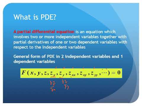
Persamaan Diferensial Parsial (Pengertian, Definisi, dan Klasifikasi)
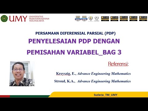
PENYELESAIAN PDP DENGAN PEMISAHAN VARIABEL BAG 3
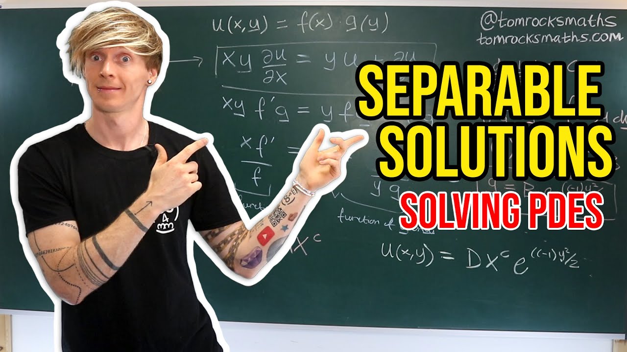
Oxford Calculus: Separable Solutions to PDEs

A concept of Differential Equation
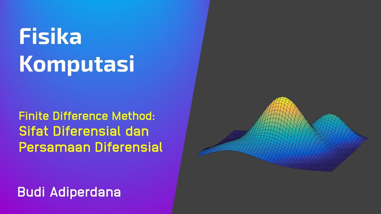
Fisika Komputasi - Metode Finite Difference 05 Sifat Diferensial dan Persamaan Diferensial
Separation of Variables // Differential Equations
5.0 / 5 (0 votes)