Sampling Theorem

Neso Academy
16 Apr 201820:35

Summary

TLDRThis lecture delves into the concept of sampling and the Sampling Theorem, crucial for understanding the transition from continuous-time to discrete-time signals in digital systems. It explains that real-life signals are analog, but digital systems require their conversion to discrete signals. The process involves multiplying a band-limited continuous-time signal by a periodic impulse train, creating a sampled signal. The lecture emphasizes the importance of the sampling frequency being at least twice the maximum frequency component of the original signal to avoid overlapping in the frequency domain, which is essential for accurate signal recovery. The Sampling Theorem is encapsulated as the condition for signal recovery from its samples, underlining the significance of using band-limited signals to prevent overlapping and ensure accurate signal reconstruction.

Takeaways

  • ๐Ÿ“š The lecture introduces the concept of sampling and the Sampling Theorem, focusing on the transition from continuous-time to discrete-time signals.
  • ๐ŸŒ The necessity to study discrete-time signals arises from the extensive use of digital technologies, which require conversion of analog, continuous-time signals to a format they can process.
  • ๐Ÿ” Sampling is defined as the process of converting a continuous-time signal into a discrete-time signal, which is essential for digital systems to handle analog information.
  • ๐Ÿ“ถ The script assumes the use of band-limited signals for sampling, which have a finite range of frequencies in their Fourier transform, simplifying the reconstruction process.
  • ๐Ÿ”ข The maximum frequency component of the message signal is denoted as Omega M and plays a crucial role in determining the conditions for signal reconstruction.
  • ๐Ÿ”„ The sampling process involves multiplying the continuous-time signal by a periodic impulse train, represented as CT, which has a fundamental period equal to the sampling interval T_s.
  • ๐Ÿ“ˆ The Fourier transform of the sampled signal, S(ฮฉ), can be found by convolving the Fourier transforms of the message signal M(ฮฉ) and the impulse train C(ฮฉ).
  • ๐Ÿ” The spectrum of the sampled signal consists of repeated images of the message signal's spectrum, shifted by integer multiples of the sampling frequency Omega S.
  • ๐Ÿšซ The condition for accurate signal recovery from its samples is that the sampling frequency (Omega S) must be greater than twice the maximum frequency component of the message signal (Omega M), preventing spectral overlap.
  • ๐Ÿ“‰ If the sampling frequency is less than twice the maximum frequency, overlapping occurs in the frequency domain, making it impossible to accurately recover the original continuous-time signal.
  • ๐Ÿ“š The Sampling Theorem concludes that a band-limited signal can be fully represented by its samples and reconstructed when the sampling frequency meets the specified condition.

Q & A

  • What is the primary reason we study discrete-time signals despite having continuous-time signals?

    -The primary reason is the extensive use of digital technologies in today's world. Since all real-life signals are analog or continuous in nature, and digital systems cannot process them directly, it is necessary to convert continuous-time signals to discrete-time signals for processing.

  • Define sampling in the context of signal processing.

    -Sampling is the process of reducing a continuous-time signal to a discrete-time signal, which can be processed by digital systems.

  • Why is it important to consider band-limited signals when discussing sampling?

    -Band-limited signals are important because their Fourier transform or spectrum is nonzero only within a finite range of frequencies. This property is crucial for accurately extracting the continuous-time signal from the sampled discrete-time signal.

  • What is the significance of the maximum frequency component (ฮฉM) of a message signal?

    -ฮฉM is significant because it represents the highest frequency component of the message signal. It is used to determine the relationship with the sampling frequency (ฮฉS) and to ensure that the sampled signal can be accurately recovered from its samples.

  • What is a sampler in the context of signal processing?

    -A sampler is a device that acts as a multiplier, taking a continuous-time signal and a periodic impulse train as inputs, and producing a sampled signal as output.

  • What is the relationship between the sampling period (Ts) and the sampling frequency (ฮฉS)?

    -The sampling frequency (ฮฉS) is the reciprocal of the sampling period (Ts). It is calculated as ฮฉS = 2ฯ€/Ts.

  • How does the spectrum of the sampled signal (ST) relate to the spectrum of the message signal (MT) and the impulse train (CT)?

    -The spectrum of the sampled signal (ST) is obtained by convoluting the spectrum of the message signal (MT) with the spectrum of the impulse train (CT) and then dividing by 2ฯ€.

  • What is the condition for accurately recovering the continuous-time signal from its sampled signal?

    -The condition for accurate recovery is that the sampling frequency (ฮฉS) must be greater than or equal to twice the maximum frequency component (ฮฉM) of the message signal.

  • What is the sampling theorem?

    -The sampling theorem states that a signal can be represented by its samples and accurately recovered if the sampling frequency is greater than or equal to twice the maximum frequency component of the signal.

  • What happens when the sampling frequency is less than twice the maximum frequency component of the signal?

    -When the sampling frequency is less than twice the maximum frequency component, overlapping occurs in the frequency spectrum, which prevents accurate recovery of the continuous-time signal from its samples.

  • Why is it necessary to avoid overlapping in the frequency spectrum when sampling a signal?

    -Avoiding overlapping is necessary to ensure that each frequency component of the original signal can be uniquely identified in the sampled signal, allowing for accurate recovery of the original signal from its samples.

  • What is the role of the guard band in the frequency spectrum of a sampled signal?

    -The guard band is the gap between the shifted versions of the message signal's spectrum in the sampled signal. It ensures that there is no overlapping, which is crucial for the accurate recovery of the original signal from its samples.

Outlines

00:00

๐Ÿ“š Introduction to Sampling and Sampling Theorem

This paragraph introduces the concept of sampling and the sampling theorem. It explains the necessity of studying discrete-time signals in the digital era, despite the prevalence of continuous-time signals in real life. The process of converting a continuous-time signal to a discrete-time signal is defined as sampling. The importance of band-limited signals is highlighted, as their Fourier transform is nonzero only within a finite range of frequencies. This property is crucial for the reconstruction of the original signal from its samples. The concept of the maximum frequency component (ฮฉ_M) is introduced, which will be frequently used throughout the course.

05:03

๐Ÿ”ข Sampling Process and the Resultant Signal

The second paragraph delves into the process of sampling, where a continuous-time signal is multiplied by a periodic impulse train to create a sampled signal. The properties of the impulse train are described, including its fundamental time period (T_s) and the associated sampling frequency (ฮฉ_s). The multiplication of the message signal (M_T) with the impulse train results in a new signal, where each impulse carries the weight of the instantaneous value of M_T at that specific time. The Fourier transform of the sampled signal is then discussed, emphasizing the convolution of the Fourier transforms of the message signal and the impulse train.

10:04

๐Ÿ“ˆ Fourier Transform of the Sampled Signal

This paragraph focuses on obtaining the Fourier transform of the sampled signal. It outlines the convolution properties used to simplify the expression for the Fourier transform of the sampled signal. The result is an expansion that includes the message signal's spectrum shifted by integer multiples of the sampling frequency (ฮฉ_s). The discussion leads to a visual representation of the spectrum, emphasizing how the spectrum appears when there is no overlapping of the shifted signal components.

15:06

๐Ÿ”‘ The Sampling Theorem and Its Conditions

The fourth paragraph explains the conditions under which the original continuous-time signal can be accurately recovered from its samples. It describes the relationship between the sampling frequency (ฮฉ_s) and the maximum frequency component of the message signal (ฮฉ_M). The sampling theorem states that accurate recovery is possible when the sampling frequency is greater than or equal to twice the maximum frequency of the signal. Two scenarios are discussed: one where there is a gap between the shifted signal components, and another where the components touch without overlapping. The possibility of overlapping, which prevents accurate recovery, is also explained.

20:08

๐Ÿšซ Limitations of Non-Band-Limited Signals

The final paragraph addresses the limitations when dealing with non-band-limited signals. It emphasizes that such signals cannot be accurately recovered from their samples due to overlapping in the frequency domain. The importance of considering band-limited signals to avoid overlapping and ensure signal recovery is reiterated. The lecture concludes with a summary of the key points and a look forward to the next lecture.

Mindmap

Keywords

๐Ÿ’กSampling

Sampling is the process of converting a continuous-time signal into a discrete-time signal, which is a fundamental concept in the video. It is essential for understanding how analog signals are transformed into a format that can be processed by digital systems. The script mentions that 'sampling is the process of reduction of a continuous time signal to a discrete time signal', illustrating its importance in the context of digital signal processing.

๐Ÿ’กSampling Theorem

The Sampling Theorem is a key principle discussed in the video that dictates the conditions under which a continuous-time signal can be accurately recovered from its samples. It states that the sampling frequency must be at least twice the maximum frequency component of the signal. The script refers to this theorem when explaining that 'a signal can be represented in its samples... and can be recovered back when the sampling frequency is greater than or equal to twice of maximum frequency component present in the signal'.

๐Ÿ’กContinuous-Time Signal

A continuous-time signal is a type of signal that can take on any value at any point in time and is naturally occurring in real life. In the video, it is mentioned that 'all real life signals are analog in nature or you can say all real life signals are continuous in nature', emphasizing the prevalence of continuous-time signals in everyday analog systems.

๐Ÿ’กDiscrete-Time Signal

A discrete-time signal is a signal that is sampled at discrete time intervals and is used in digital systems. The script explains the transition from continuous-time to discrete-time signals as 'the process of conversion or you can say, reduction of continuous time signal to discrete time signal is known as sampling', highlighting the transformation necessary for digital processing.

๐Ÿ’กDigital Technologies

Digital technologies are electronic systems that process information in discrete form rather than as a continuous signal. The video script discusses the 'extensive use of digital technologies nowadays', indicating why the study of discrete-time signals is relevant, as these technologies are prevalent in modern society.

๐Ÿ’กBand-Limited Signal

A band-limited signal is one whose frequency spectrum is confined within a finite range of frequencies. The script defines it by stating that 'band limited signal means its Fourier transform... will be nonzero only within a small range of frequencies'. This property is crucial for the sampling process because it prevents overlapping in the frequency domain, which is necessary for signal recovery.

๐Ÿ’กFourier Transform

The Fourier Transform is a mathematical technique used to convert a time-domain signal into its frequency-domain representation. In the context of the video, it is used to analyze the properties of the continuous-time signal, as mentioned when the script refers to 'the Fourier transform or you can say the spectrum of the signal'.

๐Ÿ’กMaximum Frequency Component (Omega M)

Omega M represents the highest frequency component of a message signal in the video. It is a critical parameter in the Sampling Theorem, as the script explains that 'Omega M will be used a lot in this course so remember what it is, it is the maximum frequency component of the message signal'. It helps determine the sampling frequency required for signal recovery.

๐Ÿ’กSampling Frequency (Omega S)

Omega S, or the sampling frequency, is the frequency at which a continuous-time signal is sampled in a digital system. The script describes it as 'the angular frequency of this periodic impulse train' and emphasizes its relationship with the maximum frequency component, stating that 'we are going to get relation between these two frequencies only'.

๐Ÿ’กPeriodic Impulse Train

A periodic impulse train is a series of equally spaced delta functions that serve as the sampling function in signal processing. The script describes it as 'this periodic impulse train is having the fundamental time period equal to Ds', which is used to sample the continuous-time signal and create the discrete-time signal.

Highlights

Introduction to sampling and the sampling theorem in the context of transitioning from continuous-time to discrete-time signals.

The necessity of studying discrete-time signals due to the prevalence of digital technology in processing analog signals.

Definition of sampling as the process of converting a continuous-time signal to a discrete-time signal.

Condition for recovering the continuous-time signal from the discrete-time signal.

Assumption of the message signal being band-limited for the sampling process.

Explanation of a band-limited signal and its importance in avoiding overlapping in the frequency domain.

Importance of Omega M, the maximum frequency component of the message signal, in the sampling process.

Introduction of the sampler device and its function as a multiplier in the sampling process.

Description of the periodic impulse train and its relation to the sampling frequency.

The process of obtaining the spectrum of the sampled signal through Fourier transform.

Convoluting the Fourier transform of the message signal with that of the impulse train.

The relationship between the sampling frequency (Omega s) and the maximum frequency component (Omega M).

Conditions for avoiding overlapping in the frequency spectrum and the concept of the guard band.

The critical condition for signal recovery: the sampling frequency must be greater than or equal to twice the maximum frequency component.

Illustration of the consequences of not meeting the sampling theorem condition, leading to overlapping and signal recovery issues.

The final statement of the sampling theorem and its significance in digital signal processing.

Example to demonstrate the importance of considering band-limited signals to prevent overlapping in the frequency domain.

Conclusion of the lecture with a summary of the key points and an invitation to the next lecture.

Transcripts

play00:00

in this lecture we will understand what

play00:02

do we mean by sampling and what is

play00:05

sampling theorem till now we have done a

play00:09

lot of discussions on continuous-time

play00:11

signals and now it's time to move on to

play00:15

discrete-time signals but wait why we

play00:19

are required to study the concepts

play00:21

related to discrete-time signals when we

play00:24

already have continuous-time signals the

play00:27

answer is extensive use of digital

play00:30

technologies nowadays so if you look

play00:33

around yourself you will find there are

play00:36

so many digital technologies in

play00:39

implementation but we know all real life

play00:42

signals are analog in nature or you can

play00:45

say all real life signals are continuous

play00:48

in nature so they are continuous time

play00:51

signals so the information is carried by

play00:55

continuous time signal but the systems

play00:59

we are using our digital in nature

play01:02

therefore they will not process

play01:04

continuous time signal and it becomes

play01:07

important to convert the continuous time

play01:10

signal to discrete time signal and this

play01:15

process of conversion or you can say

play01:18

reduction of continuous time signal to

play01:21

discrete time signal is known as

play01:24

sampling now let us define sampling

play01:28

properly sampling is the process of

play01:31

reduction of a continuous time signal to

play01:35

a discrete time signal and if you want

play01:39

to get the continuous time signal back

play01:42

from the discrete time signal then you

play01:46

can do this but there is some condition

play01:49

and now we will try to obtain that

play01:51

particular condition so let's move on to

play01:55

the next part of this lecture let us

play01:58

take one continuous time signal and

play02:00

let's say we want to convert this

play02:02

continuous time signal to a discrete

play02:04

time signal and we are representing this

play02:08

continuous time signal by M T and

play02:12

representing it by empty because this

play02:15

signal is known as message signal this

play02:20

is known as message signal because this

play02:24

signal is carrying the information we

play02:27

want to process and you must note one

play02:30

point here this signal we have taken is

play02:33

a band limited signal we are assuming

play02:37

that we have taken a continuous-time

play02:40

signal which is a band limited signal

play02:45

now why we are taking band limited

play02:48

signal and what is band limited signal I

play02:51

will explain now band limited signal

play02:54

means its Fourier transform or you can

play02:57

say the spectrum of the signal will be

play03:00

nonzero only within a small range of

play03:04

frequencies for example let's say this

play03:07

signal is having the Fourier transform M

play03:10

Omega like this now you can see that the

play03:14

Fourier transform or the spectrum is non

play03:17

zero from minus Omega M 2 plus Omega M

play03:21

so here in this case we are having the

play03:24

spectrum which is nonzero only for a

play03:27

finite range of frequencies and it will

play03:30

be very helpful when we will try to

play03:33

extract the continuous-time signal from

play03:36

the converted discrete-time signal and

play03:39

this point will be more clear after some

play03:42

time so for now just understand that we

play03:45

are having a continuous-time signal

play03:47

carrying the message and his Fourier

play03:50

transform is like this and the Fourier

play03:54

transform is nonzero between minus Omega

play03:57

M and Omega M and also note down what is

play04:02

Omega M Omega M is the maximum maximum

play04:09

frequency component of the message

play04:15

signal MT Omega M will be used a lot in

play04:19

this course so remember what it is it is

play04:21

the maximum frequency component of

play04:24

empty if empty is having multiple

play04:27

frequency components then the maximum

play04:29

frequency out of those frequency

play04:32

components is Omega M in the next

play04:35

lecture we will solve numerical problem

play04:38

and there this point will be more clear

play04:41

now we will move on to the next process

play04:43

and the next process is feeding this

play04:47

continuous-time signal to a device known

play04:50

as sampler now this device sampler is

play04:54

simply acting as multiplier it is acting

play04:59

as multiplier and multiplier means it is

play05:03

going to multiply to continuous-time

play05:06

signals first signal is empty and the

play05:09

second signal is CT and you can clearly

play05:13

see that Ct is a periodic impulse train

play05:16

and this periodic impulse train is

play05:19

having the fundamental time period equal

play05:22

to D s so T s is the fundamental time

play05:27

period or it is the sampling period it

play05:31

is also known as sampling period it is

play05:39

also known as sampling interval it is

play05:44

also known as sampling interval and we

play05:50

know Omega s which is the angular

play05:53

frequency is equal to 2 pi divided by T

play05:59

s and Omega s is known as the sampling

play06:02

frequency it is known as the sampling

play06:06

frequency so now we have two frequencies

play06:10

the first frequency is Omega M known as

play06:13

the maximum frequency component of MT

play06:16

and the another frequency we have is

play06:19

Omega s which is the sampling frequency

play06:22

or the angular frequency of this

play06:25

periodic impulse train and remember both

play06:29

the frequencies because we are going to

play06:31

get relation between these two

play06:34

frequencies only and as we are having

play06:37

the periodic impulse train like this we

play06:40

can write it as summation and equal to

play06:46

minus infinity to infinity Delta t minus

play06:50

n TS now when n is equal to 0 we will

play06:55

have Delta T this means impulse present

play06:58

at the origin when n is equal to 1 we

play07:01

will have Delta t minus TS this means

play07:04

the unit impulse which is present at TS

play07:08

simply shift the unit impulse present at

play07:11

the origin towards the right by TS and

play07:14

you will have delta t minus t s so this

play07:17

impulse you are looking here is delta t

play07:20

minus TS this impulse is delta T this

play07:23

impulse is delta t plus TS and we will

play07:27

have it when n is equal to minus 1

play07:29

similarly we will have all the other

play07:31

impulses and we will have the impulse

play07:34

train like this now after multiplying

play07:37

empty and CT we will have the resultant

play07:41

waveform like this in this waveform we

play07:45

are having different impulses and the

play07:47

area or weight of the impulse is equal

play07:50

to the instantaneous value of signal MT

play07:54

for example if you talk about the

play07:58

impulse present at T s then this impulse

play08:01

will have the weight or strength equal

play08:04

to the instantaneous value of M T this

play08:08

means when T is equal to T s the value

play08:12

of M T will be the strength or weight of

play08:15

this particular impulse and in this way

play08:18

we have a new signal which is known as

play08:22

sampled signal and represented by as T s

play08:27

T is equal to empty message signal

play08:31

multiplied to the periodic impulse train

play08:34

C T and now we are interested in

play08:37

obtaining the spectrum of the sampled

play08:42

signal this means we are having s T and

play08:45

we want to have the Fourier transform as

play08:49

Omega of

play08:51

steal and we also know that s T is equal

play08:55

to message signal multiplied to the

play08:58

periodic impulse train CT and we know

play09:01

the property of Fourier transform when

play09:04

two signals are multiplied if you try to

play09:09

take the Fourier transform then on the

play09:13

left hand side you will have the Fourier

play09:15

transform of this signal which is s

play09:19

Omega and on the right hand side you

play09:21

will have 1 divided by 2 pi multiplied

play09:25

to the Fourier transform of Mt which is

play09:29

M Omega convoluted with the Fourier

play09:34

transform of CT and let's say Fourier

play09:38

transform of CD

play09:39

is C Omega so we can easily obtain the

play09:44

Fourier transform as Omega after

play09:46

convoluting M Omega and C Omega and then

play09:49

dividing it by 2 pi M Omega we have

play09:53

assumed here but what about C Omega if

play09:57

you remember in the Fourier transform

play09:59

solved problem number 11 we solved one

play10:03

problem in which the time domain signal

play10:06

was exactly like this and we obtained

play10:10

the Fourier transform of this signal and

play10:13

the result we got was equal to Omega s

play10:19

summation n equal to minus infinity to

play10:23

infinity Delta Omega minus n Omega s so

play10:30

we have C Omega and we have M Omega now

play10:33

let's move on to the simplification of

play10:36

this and in order to simplify this we

play10:40

need to use the properties of

play10:42

convolution and the properties of

play10:45

impulse signal we are having as Omega as

play10:49

Omega equal to 1 over 2 pi 1 over 2 pi

play10:56

multiplied to M Omega M Omega

play11:01

convolution with C Omega and Co

play11:04

is equal to this so we will write Omega

play11:07

as summation and equal to minus infinity

play11:12

to infinity Delta Omega minus and Omega

play11:17

s and we can take this Omega s outside

play11:21

then we will have s Omega equal to Omega

play11:25

s divided by 2 pi inside the bracket M

play11:29

Omega convolution with summation and

play11:34

equal to minus infinity to infinity

play11:37

Delta Omega minus and Omega s and we

play11:42

know Omega s divided by 2 pi will be

play11:45

equal to 1 over TS from here you can see

play11:49

that Omega s divided by 2 pi will be

play11:52

equal to 1 over TS

play11:54

so in the next step we will write Omega

play11:57

s divided by 2 pi equal to 1 over TS and

play12:01

inside the bracket we can rearrange this

play12:04

and we can write summation n equal to

play12:08

minus infinity to infinity M Omega M

play12:12

Omega convolution who with Delta Omega

play12:17

minus n Omega s and we know the property

play12:21

by which we can simplify this further

play12:24

and according to the property if we have

play12:28

a signal XT and the signal is convoluted

play12:31

with Delta t minus T 1 then this is

play12:35

equal to X t minus T 1 we simply need to

play12:41

put t minus t 1 in place of T and if we

play12:45

follow this we will put Omega minus n

play12:49

Omega s in place of this Omega so in the

play12:52

next step we will have s Omega equal to

play12:57

1 divided by TS inside the bracket

play13:01

summation and equal to minus infinity to

play13:05

infinity M Omega minus n Omega s M Omega

play13:11

minus n Omega s this is what we need and

play13:15

now let X

play13:17

and this by putting the different values

play13:20

of n so we will have as Omega equal to 1

play13:25

divided by TS inside the bracket when n

play13:30

is equal to 0 we will have M Omega we

play13:33

will have M Omega and we have the wave

play13:37

form of M Omega now when n is equal to 1

play13:41

we will have M Omega minus Omega s so we

play13:45

will have M Omega minus Omega s

play13:50

similarly we will have different terms

play13:52

when n is equal to minus 1 we will have

play13:56

ham Omega plus Omega s we will have M

play14:00

Omega plus Omega s similarly for

play14:05

negative values of n we will have

play14:07

different terms so in this way we are

play14:10

getting the expansion of has Omega and

play14:14

using this expansion we can plot the

play14:17

wave form of s Omega and the wave form

play14:20

will look like this if you refer the

play14:23

expansion you will find when n is equal

play14:27

to 0 we are having M Omega this means we

play14:32

should have this wave form and therefore

play14:34

this wave form here is the wave form of

play14:38

M Omega this makes this frequency equal

play14:43

to minus Omega m and this frequency

play14:45

equal to Omega M and when n is equal to

play14:49

1 we are having M Omega minus Omega s

play14:54

this means M Omega has shifted towards

play14:58

the right by Omega s this makes this

play15:02

frequency here this frequency equal to

play15:05

Omega s minus Omega M this frequency

play15:10

here equal to Omega M plus Omega s or

play15:15

you can write Omega S Plus Omega M and

play15:17

this particular frequency here equal to

play15:21

Omega s now you can notice one thing

play15:23

that Omega s minus Omega M is greater

play15:27

than Omega M

play15:29

Omega s minus Omega M is greater than

play15:34

Omega M this implies we are getting

play15:36

omega s greater than twice of Omega M so

play15:42

when Omega S which is the sampling

play15:45

frequency greater than twice of maximum

play15:49

frequency component of the message

play15:51

signal then there is no overlapping in

play15:55

this spectrum by no overlapping I mean

play15:58

this triangle and this triangle are not

play16:01

overlapping there is sufficient gap

play16:04

between the two triangles and this gap

play16:07

here this gap here is known as guard

play16:12

band now what will happen when Omega s

play16:16

minus Omega m is equal to Omega M this

play16:19

means this frequency here which is Omega

play16:23

M is equal to this frequency here which

play16:25

is omega s minus Omega M it is very

play16:29

obvious that the triangles will be

play16:32

touching so you will have the waveform

play16:34

like this when Omega s minus Omega M is

play16:38

equal to Omega M or you can say Omega s

play16:42

is equal to twice of Omega M now in the

play16:46

two scenarios we have discussed till now

play16:49

we can recover the continuous-time

play16:52

signal from the sampled signal because

play16:55

there is no overlapping in the first

play16:58

case there is a gap and hence there is

play17:01

no overlapping in the second case they

play17:04

are touching and again there is no

play17:06

overlapping but if there is overlapping

play17:09

then we cannot recover the

play17:11

continuous-time signal accurately now

play17:14

let's try to understand in what

play17:16

condition the overlapping will occur we

play17:19

have discussed the first case in which

play17:21

we found when Omega s is greater than

play17:24

twice of Omega

play17:26

there will be gap and when Omega s is

play17:29

equal to twice of Omega M there will be

play17:32

touching case and when Omega s is less

play17:36

than twice of Omega M

play17:38

when Omega s is less than twice of Omega

play17:41

M then there will be overlapping as you

play17:44

can see on your screen and you can

play17:47

understand the point that Omega s minus

play17:50

Omega is less than Omega M this makes

play17:54

the overlapping possible and in this

play17:57

scenario you cannot recover the

play17:59

continuous-time signal accurately and

play18:02

this is known as sampling theorem so

play18:06

let's move on to the final statement of

play18:10

sampling theorem

play18:11

according to sampling theorem a signal

play18:15

can be represented in its samples like

play18:18

we have done we have represented signal

play18:21

MT in its samples which is sampled

play18:27

signal st and can be recovered back when

play18:31

the sampling frequency this means omegas

play18:34

is greater than or equal to twice of

play18:38

maximum frequency component present in

play18:41

the signal this means twice of Omega M

play18:45

so when omegas is greater or equal to

play18:49

twice of Omega M we can recover back the

play18:51

signal from its samples so remember this

play18:55

condition omegas should be greater or

play18:59

equal to twice of Omega M this is a very

play19:03

important condition so this is all for

play19:07

the sampling theorem and initially I

play19:10

told you that we are considering the

play19:13

band limited signal we considered our

play19:16

message signal to be band limited signal

play19:19

to get before you transform like this

play19:22

and we are getting the Fourier transform

play19:25

like this because we don't want the

play19:28

overlapping now we will try to

play19:30

understand this point by the help of one

play19:33

example and in this example we are

play19:36

considering the time domain signal has

play19:39

not band-limited and as the time domain

play19:43

signal is not band limited the Fourier

play19:47

transform will not be bounded like this

play19:49

it will be something like this now

play19:53

repeat this structure like this and you

play19:57

will find there is over lapping and we

play20:00

are trying to avoid the overlapping so

play20:02

that we can recover the time domain

play20:04

signal from its samples but if you take

play20:08

the not band-limited signal you will

play20:11

have the overlapping and therefore

play20:13

recovery will not be possible and this

play20:15

is the reason we are taking the

play20:18

band-limited

play20:19

signal and this is all for this lecture

play20:22

see you in the next one

play20:24

[Applause]

play20:27

[Music]

Rate This
โ˜…
โ˜…
โ˜…
โ˜…
โ˜…

5.0 / 5 (0 votes)

Related Tags
Signal ProcessingSamplingDigital TechnologyContinuous-TimeDiscrete-TimeBand-LimitedFourier TransformSampling FrequencySignal RecoveryLecture Series