Learning Decision Tree

Machine Learning- Sudeshna Sarkar
28 Jun 201629:24

Summary

TLDRThe transcript discusses the process of decision tree algorithm design, focusing on the importance of attribute selection and example classification. It explains the concept of entropy and its role in determining the purity of a set, guiding the decision-making process in tree splitting. The speaker illustrates how to assess the performance of different attributes using entropy and information gain, emphasizing the goal of maximizing information gain to improve classification accuracy. The summary also touches on the practical application of these concepts in building an optimal decision tree model.

Takeaways

  • 🌟 The discussion begins with a review of the decision tree algorithm and its foundational structure.
  • 🔍 The script introduces the concept of using 'd' as a group of decision examples and 'A' as attributes, with two children of 'A' being considered.
  • 📊 It explains the process of determining a decision tree by identifying the best attributes to split the data, starting with 'A' and then dividing 'D' into 'D1' and 'D2'.
  • 📈 The script discusses the importance of entropy in decision-making within the tree, using examples to illustrate how to calculate and apply it.
  • 🔑 The concept of choosing the best attribute to split the data is emphasized, with a focus on minimizing entropy.
  • 📉 The script provides a method to decide when to stop splitting, considering various scenarios and conditions.
  • 💡 It introduces the idea of using information gain to select the best attribute, explaining how it can be calculated and used to make decisions.
  • 📝 The script explains how to handle continuous attributes in decision trees, suggesting methods for discretization.
  • 🔎 The process of building a decision tree is outlined, including the use of examples to illustrate the steps involved.
  • 📚 The script concludes with a summary of the decision tree construction process, emphasizing the importance of understanding the underlying principles and calculations.

Q & A

  • What does the speaker suggest to start with when discussing decision trees?

    -The speaker suggests starting with the concept of 'd', which is a group of examples for decision trees, and then moving on to identify 'A' as the attribute to consider, with two children of 'A' and examples for 'D' that are initially related to 'A'.

  • How does the speaker propose to decide on the division of 'D' into 'D1' and 'D2'?

    -The speaker proposes to consider a specific branch as equivalent to 'A', meaning that 'D1' would contain examples equivalent to 'A1', which are similar to 'A', and 'D2' would contain examples equivalent to 'A2', which are similar to 'A' being false.

  • What is the significance of the examples in 'D1' and 'D2' according to the speaker?

    -The examples in 'D1' are significant as they are equivalent to 'A1', which is similar to 'A', and the examples in 'D2' are significant as they are equivalent to 'A2', which is similar to 'A' being false.

  • What is the purpose of the decision-making process described in the script?

    -The purpose of the decision-making process is to determine the best attribute to split on in a decision tree, considering the entropy and information gain at each step.

  • How does the speaker suggest making decisions about which attribute to split on?

    -The speaker suggests making decisions by considering the number of features that need to be nullified, and by looking at the attributes that are most significant in reducing entropy.

  • What is the role of entropy in the decision-making process as described in the script?

    -Entropy plays a crucial role in the decision-making process as it helps in determining the purity of the classes. The goal is to minimize entropy by choosing the attribute that best splits the data into classes with high purity.

  • How does the speaker explain the concept of information gain in the context of decision trees?

    -The speaker explains information gain as the reduction in entropy after a split. It is calculated by comparing the entropy of the parent node to the weighted average entropy of the child nodes resulting from the split.

  • What is the significance of the attribute 'A1' in the decision tree example provided by the speaker?

    -The attribute 'A1' is significant because it is used to further split the data and is considered to have a higher information gain, leading to a more informative decision tree.

  • How does the speaker use the concept of 'entropy' to decide on the splits in the decision tree?

    -The speaker uses the concept of 'entropy' to decide on the splits by calculating the entropy of the examples in each branch and choosing the split that results in the lowest entropy, indicating a more informative split.

  • What does the speaker mean by 'majority voting' in the context of decision trees?

    -The speaker refers to 'majority voting' as a method where the class label is determined by the majority of the training examples in each node of the decision tree.

  • How does the speaker suggest improving the decision tree model?

    -The speaker suggests improving the decision tree model by continuously identifying and splitting on the attributes that provide the highest information gain and lowest entropy.

Outlines

00:00

🌟 Introduction to Decision Tree Algorithm

The paragraph introduces the concept of revisiting the design tree algorithm, starting with several examples of decision-making. The focus is on identifying attributes such as 'A' which are considered as the root of the decision tree, and then further dividing into 'D1' and 'D2'. It explains the process of categorizing examples into 'D1' and 'D2' based on their similarity to 'A', and how this division is used to make decisions. The paragraph also discusses the process of making decisions based on the division, considering various scenarios and how to handle them.

05:02

🔍 Decision Making Process and Entropy

This paragraph delves into the decision-making process using the decision tree, emphasizing the importance of entropy in determining the best attribute to split the data. It discusses how to decide which attribute to use for splitting based on the information gain and how entropy plays a crucial role in this decision. The concept of entropy is explained, and its significance in classifying data into classes is highlighted. The paragraph also touches upon the use of entropy to measure the impurity of a dataset and how it guides the splitting process.

10:11

📊 Entropy and Information Gain in Decision Trees

The paragraph explains the mathematical concept of entropy in the context of decision trees, describing it as a measure of uncertainty or disorder in a dataset. It discusses how entropy is calculated and its role in determining the best split in a decision tree. The concept of information gain is introduced, which is the difference in entropy before and after a split, and how it is used to select the attribute that results in the highest information gain. The paragraph also provides an example of how entropy values are used to make decisions about which attribute to split on.

15:14

📈 Analyzing Entropy and Decision Tree Splits

This paragraph continues the discussion on entropy and its application in decision trees, focusing on how to analyze the entropy of different attributes to decide the best split. It provides an example where the entropy of different attributes is calculated, and a decision is made based on which attribute provides the highest information gain. The paragraph also discusses the concept of using a threshold to decide whether to split further or not, based on the calculated entropy and information gain.

20:33

🌐 Applying Decision Trees to Real-world Scenarios

The paragraph illustrates the application of decision tree algorithms to real-world scenarios, such as predicting weather conditions. It discusses how to use the decision tree to make predictions based on various attributes like temperature, humidity, and wind. The concept of information gain is applied to choose the best attribute for splitting the data, leading to more accurate predictions. The paragraph also touches upon the process of refining the decision tree and using it for continuous attribute identification.

25:35

🔧 Conclusion and Future Steps in Decision Tree Analysis

In the concluding paragraph, the speaker summarizes the discussion on decision trees, emphasizing the importance of understanding the algorithm and its applications. It mentions the computational intensity of decision tree analysis and the need for computational tools to handle it efficiently. The paragraph also hints at future discussions on decision tree algorithms, suggesting that the audience can expect further exploration of the topic in subsequent sessions.

Mindmap

Keywords

💡Decision Tree

A decision tree is a flowchart-like structure in which each internal node represents a 'test' on an attribute, each branch represents the outcome of the test, and each leaf node represents a class label (decision taken after computing all attributes). In the script, the decision tree is used to classify examples based on various attributes, starting with 'A' and then branching out to 'D1' and 'D2', illustrating the process of decision-making through a structured and hierarchical model.

💡Entropy

Entropy, in the context of the video, is a measure of the impurity or disorder within a dataset. It is used to quantify the uncertainty or the expected information content of a random variable. The script discusses entropy in relation to decision trees, where the goal is to select attributes that maximize the information gain and thus reduce entropy, leading to a more efficient classification.

💡Information Gain

Information gain is a concept used in decision trees to select the best attribute to split the data. It measures the reduction in entropy brought about by splitting the dataset according to a particular attribute. The script mentions information gain when discussing how to choose the best attribute to split the data, aiming to find the attribute that results in the highest information gain, thus leading to a more informative and efficient decision tree.

💡Attribute

An attribute in the video script refers to a specific characteristic or property of the data points being analyzed. Attributes are used to make decisions in the decision tree, with examples like 'A', 'D1', and 'D2' being considered for splitting the data. The choice of attribute is crucial as it determines the branches of the tree and ultimately the classification of the data.

💡Classification

Classification is the process of predicting the category or class of an entity based on its features. In the script, classification is the main goal of building a decision tree, where the data is divided into classes such as 'A1', 'A2', 'D1', 'D2', etc. The video discusses how to improve classification accuracy by choosing the right attributes and splits.

💡Splitting

Splitting in the context of the video refers to the process of dividing the dataset into subsets based on the values of an attribute. This is a key operation in building a decision tree, as it helps in creating branches that lead to more homogeneous subsets, which are easier to classify. The script describes how to decide when to split the data and how to choose the best attribute for splitting.

💡Examples

In the video, examples refer to the individual data points or instances that are being classified by the decision tree. The script discusses how the decision tree is built to handle examples, with a focus on how the tree structure helps in classifying these examples more accurately based on their attributes.

💡Gini Index

The Gini index, mentioned in the script, is a measure of inequality or impurity in a dataset. It is used in decision tree algorithms to select the attribute that most reduces the impurity of the child nodes. The lower the Gini index, the more homogeneous the dataset is. The script discusses how to calculate the Gini index and use it to evaluate potential splits in the decision tree.

💡Pruning

Pruning is the process of removing parts of the decision tree to prevent overfitting. Overfitting occurs when the tree is too complex and fits the training data too closely, which can lead to poor generalization to new data. The script touches upon the concept of pruning as a way to simplify the tree and improve its performance on unseen data.

💡Root Node

The root node in a decision tree is the topmost node from which the tree grows. In the script, the root node is used to start the decision-making process, with subsequent nodes branching out based on attribute values. The choice of the root node is important as it sets the initial direction for the tree's structure and classification.

💡Leaf Node

A leaf node, as discussed in the script, is an endpoint of a branch in the decision tree that does not lead to any further nodes. It represents a final decision or classification. The script explains how leaf nodes are determined based on the attributes and the splits made in the tree, with the goal of reaching a classification decision at each leaf node.

Highlights

Introduction to Decision Tree Algorithm and its basic structure.

Starting with several examples of decision-making.

The concept of 'd' as a group of decision-making examples.

Desire to determine the Decision Tree and the need to identify 'A' as attributes.

Explanation of how 'A' has two children and the examples of 'D' are divided into 'D1' and 'D2'.

Assumption that a specific branch is equivalent to 'A' and its relation to 'D1'.

Discussion on how 'D1' contains examples that are similar to 'A1', and 'D2' contains examples similar to 'A2'.

Explanation of the need to make decisions at a certain point in the Decision Tree.

The process of making decisions based on the context of three features and their impact on the decision.

The concept of nullifying or eliminating certain branches based on the examples and their attributes.

The idea of considering the value of 'D1' and the implications for the Decision Tree.

Discussion on how to make decisions based on the number of examples and their distribution.

The concept of entropy and its role in decision-making within the Decision Tree.

Explanation of how to calculate entropy and its significance in the decision-making process.

The use of entropy to determine the best attribute to split the data and its impact on the Decision Tree.

The concept of information gain and its importance in selecting the best attribute for splitting.

Discussion on how to calculate information gain and its comparison with entropy.

The decision to split the 'A1' attribute further into 'A1_low', 'A1_medium', and the rationale behind it.

The process of identifying the best attribute to split based on the examples and their values.

The use of a slide to illustrate the decision-making process and the selection of the best attribute.

The concept of classifying examples based on the attribute and the resulting information gain.

The decision to use the 'A2' attribute over 'A1' due to its higher information gain.

The process of making decisions based on the attributes 'Temperature', 'Humidity', and 'Wind', and their respective information gains.

The final decision to prioritize 'Temperature' over 'Wind' based on their information gains.

The concept of using the third attribute 'Outlook' and its impact on the decision tree.

The process of calculating the information gain for 'Outlook' and its comparison with other attributes.

The decision to use all four attributes and the resulting information gain.

The process of making a final decision tree and its practical applications.

The concept of continuous attributes and how to handle them in the Decision Tree.

The process of identifying the best splits for each attribute based on information gain.

The conclusion of the lecture and the transition to the next module.

Transcripts

play00:18

ಶುಭೋದಯ. ಡಿಸಿಷನ್ ಡಿಸಿಷನ್ ಟ್ರೀ ಅಲ್ಗಾರಿದಮ್‌ನ

play00:22

ಮೂಲ ರೂಪರೇಖೆಯನ್ನು ಮರುಪರಿಶೀಲಿಸೋಣ.

play00:25

ನಾವು ಹೇಳಿದಂತೆ ನಾವು ಹಲವಾರು ತರಬೇತಿ ಉದಾಹರಣೆಗಳೊಂದಿಗೆ

play00:31

ಪ್ರಾರಂಭಿಸುತ್ತೇವೆ. ನಾವು ಕುಳಿತು d ಎಂಬುದು

play00:34

ತರಬೇತಿ ಉದಾಹರಣೆಗಳ ಗುಂಪಾಗಿದೆ. ಈಗ ನಾವು

play00:36

ಡಿಸಿಷನ್ ಟ್ರೀ ಅನ್ನು ನಿರ್ಧರಿಸಲು ಬಯಸುತ್ತೇವೆ.

play00:38

ಆದ್ದರಿಂದ, ನಾವು ಕಂಡುಹಿಡಿಯಲು ಬಯಸುತ್ತೇವೆ, A ಎಂಬುದು

play00:41

ಅಟ್ರಿಬ್ಯೂಟ್ ಗಳನ್ನು ಎಂದು ಭಾವಿಸೋಣ ಮತ್ತು

play00:44

ಅದಕ್ಕೆ ಅನುಗುಣವಾಗಿ ನಾವು A ಯ ಇಬ್ಬರು ಮಕ್ಕಳನ್ನು

play00:49

ಹೊಂದಿರುತ್ತೇವೆ ಮತ್ತು D ಅನ್ನು ಹೊಂದಿಸುವ

play00:52

ತರಬೇತಿ ಉದಾಹರಣೆಗಳನ್ನು ಹೊಂದಿದ್ದೇವೆ, ಅದು

play00:55

ಆರಂಭದಲ್ಲಿ A ಮಾರ್ಗದೊಂದಿಗೆ ಸಂಬಂಧ ಹೊಂದಿದೆ. D 1

play01:02

ಮತ್ತು D 2 ಆಗಿ ವಿಭಜಿಸಿ. ಈ ನಿರ್ದಿಷ್ಟ ಶಾಖೆಯು

play01:09

A ಗೆ ಸಮಾನವಾಗಿದೆ ಎಂದು ಭಾವಿಸೋಣ, ಇದು A ಗೆ

play01:17

ಸಮಾನವಾಗಿರುತ್ತದೆ, ಆದ್ದರಿಂದ D 1 ಆ ಉದಾಹರಣೆಗಳನ್ನು

play01:21

ಹೊಂದಿರುತ್ತದೆ, ಇದರಿಂದ A 1 ಸರಿಗೆ ಸಮಾನವಾಗಿರುತ್ತದೆ,

play01:24

D 2 ಆ ಉದಾಹರಣೆಗಳನ್ನು ಹೊಂದಿರುತ್ತದೆ ಇದು

play01:30

ಸುಳ್ಳಿಗೆ ಸಮಾನವಾಗಿರುತ್ತದೆ. ಈಗ ಈ ಪರೀಕ್ಷೆಯಲ್ಲಿ

play01:37

D 1 ಅನ್ನು ನೋಡಿದಾಗ ಈ ಹಂತದಲ್ಲಿ ಡಿಸಿಷನ್ಗೆ

play01:41

ಹೋದಾಗ ಒಬ್ಬರು ಮಾಡಬೇಕಾದ ಆಯ್ಕೆಗಳು ಇವು.

play01:45

ಈಗ ನಾವು ಆ ನಿರ್ಧಾರಗಳನ್ನು ಹೇಗೆ ತೆಗೆದುಕೊಳ್ಳುತ್ತೇವೆ

play01:50

ಎಂದು ನೋಡೋಣ. ಮೊದಲು ಯಾವಾಗ ನಿಲ್ಲಿಸಬೇಕು

play01:53

ಎಂಬ ನಿರ್ಧಾರವನ್ನು ನೋಡೋಣ.

play01:56

ನೀವು ನಿಲ್ಲಿಸಬೇಕಾದ ಹಲವಾರು ಸಂದರ್ಭಗಳಿವೆ,

play01:59

ಮೊದಲನೆಯದಾಗಿ ಮೂರು ಫೀಚರ್ ಅನ್ನು A 1 ಅನ್ನು

play02:03

ಆಯ್ಕೆ ಮಾಡಿದ್ದೀರಿ ಮತ್ತು ಅದರ ಆಧಾರದ

play02:08

ಮೇಲೆ ನೀವು A 1 ಅನ್ನು ಹೊಂದಿದ್ದೀರಿ ಮೊದಲು

play02:14

ನೀವು ಈ ವಿಭಜನೆಯನ್ನು ಪಡೆದುಕೊಂಡಿದ್ದೀರಿ

play02:17

ಮತ್ತು ನಂತರ ನೀವು A 3 ಅನ್ನು ಆಯ್ಕೆ ಮಾಡಿದ್ದೀರಿ

play02:23

ಮತ್ತು A 3 ಅನ್ನು ಸರಿಗೆ ಸಮನಾದ A 3 ಅನ್ನು ಆಧರಿಸಿ

play02:28

ನೀವು ಈ ವಿಭಜನೆಯನ್ನು ಪಡೆದುಕೊಂಡಿದ್ದೀರಿ

play02:31

ಎಂದು ಭಾವಿಸೋಣ ಮತ್ತು ಇಲ್ಲಿ ನೀವು A 2 ಅನ್ನು

play02:37

ಆಯ್ಕೆ ಮಾಡಿದ್ದೀರಿ ಮತ್ತು A 2 ಅನ್ನು ಸರಿ

play02:45

ಅಥವಾ ತಪ್ಪಿಗೆ ಸಮನಾಗಿರುತ್ತದೆ ಎಂದು ಭಾವಿಸೋಣ. ಈ ವಿಭಜನೆ.

play02:53

ಇಲ್ಲಿ ನಾವು D 2 ಅನ್ನು ಹೊಂದಿದ್ದೇವೆ ಎಂದು

play02:59

ಭಾವಿಸೋಣ, ಇಲ್ಲಿ ನಾವು D 3 ಅನ್ನು ಹೊಂದಿದ್ದೇವೆ

play03:04

ಮತ್ತು ಇಲ್ಲಿ ನಾವು D 4 ಅನ್ನು ಹೊಂದಿದ್ದೇವೆ.

play03:09

ಈಗ, ಎಲ್ಲಾ 3 ಅಟ್ರಿಬ್ಯೂಟ್ ಗಳನ್ನು ದಣಿದಿದ್ದಲ್ಲಿ

play03:17

ಇಲ್ಲಿ ನಿಲ್ಲಿಸಬೇಕು, ನಾವು ಆಯ್ಕೆಯನ್ನು

play03:23

ಹೊಂದಿದ್ದೇವೆ. D 1 ನಲ್ಲಿನ ಎಲ್ಲಾ ಉದಾಹರಣೆಗಳು

play03:27

ವ್ಯಾಲ್ಯೂ ಮತ್ತು D 5 ಎಂದು ನಾವು 2 ಎಂದು

play03:33

ಹೇಳೋಣ, ನಮಗೆ ಎರಡು ಕೆಲವು ಉದಾಹರಣೆಗಳಿವೆ

play03:37

ನಂತರ ನಾವು ನಿಲ್ಲಿಸಬೇಕು. ಇವು ಮೂರು ಸಂಭವನೀಯ

play03:42

ನಿಲ್ಲಿಸುವ ಮಾನದಂಡಗಳಾಗಿವೆ. ಮುಂದೆ ನಾವು ಯಾವ ನೋಡ್‌ನಲ್ಲಿ

play03:46

ವಿಭಜಿಸಬೇಕು ಎಂಬುದರ ಕುರಿತು ನಿರ್ಧಾರವನ್ನು

play03:49

ನೋಡುತ್ತೇವೆ, ಅದರ ಮೇಲೆ ಯಾವ ಅಟ್ರಿಬ್ಯೂಟ್

play03:53

ಚಿಕ್ಕದಾಗಿದೆ ಎಂದು ನಿರೀಕ್ಷಿಸಲಾಗಿದೆ.

play03:56

ನಾವು ಮಾಡಬಹುದಾದ ಇನ್ನೊಂದು ವಿಷಯವೆಂದರೆ ನಾವು

play03:59

ಯೋಚಿಸಬಹುದು, ನೀವು ಇಲ್ಲಿ ಉದಾಹರಣೆಗಳನ್ನು

play04:03

ಹೊಂದಿದ್ದರೆ ನಾವು D 2 ಅನ್ನು ಹೇಳೋಣ ಮತ್ತು

play04:08

ಅದು 2 ಕ್ಲಾಸ್ ಎಂದು ಹೇಳಬಹುದು ಮತ್ತು ನಂತರ

play04:13

ನಾವು ದೋಷವನ್ನು ಮಾಡಿದ್ದೇವೆ ಮತ್ತು ಆ ದೋಷವು 40 ಪ್ರತಿಶತವಾಗಿದೆ.

play04:20

ಆದ್ದರಿಂದ, ನಾವು ನಿಲ್ಲಿಸಬಹುದು ಆದ್ದರಿಂದ ವಿಭಜನೆಯು

play04:24

ಚಿಕ್ಕ ಎರರ್ ಗಳನ್ನು ಹೊಂದಿದ್ದರೆ, ಇದು

play04:27

ನಾವು ಮಾಡಬಹುದಾದ ಕೆಲಸಗಳಲ್ಲಿ ಒಂದಾಗಿದೆ ಮತ್ತು ನಾವು

play04:32

ಈ ಕುರಿತು ಹೆಚ್ಚಿನದನ್ನು ನೋಡುತ್ತೇವೆ.

play04:35

ಈಗ ಈ ಉದಾಹರಣೆಯಲ್ಲಿ ನಮ್ಮ ಅಟ್ರಿಬ್ಯೂಟ್

play04:39

ಗಳನ್ನು ಅರ್ಧಕ್ಕೆ ವಿಭಜಿಸಬಹುದು ಇದರಿಂದ

play04:42

ನಮಗೆ ಇಬ್ಬರು ಮಕ್ಕಳಿದ್ದಾರೆ.

play04:45

ಒಂದು ನಿರ್ದಿಷ್ಟ ಅಟ್ರಿಬ್ಯೂಟ್ ನಲ್ಲಿ ನಾವು ಮತ್ತೆ

play04:49

ವಿಭಜಿಸಬಹುದು ಮತ್ತು A 1 ಅನ್ನು A 1 ಕಡಿಮೆ A

play04:56

1 ಮಧ್ಯಮ ಎಂದು ಹೇಳೋಣ. ಆದ್ದರಿಂದ, ಮೌಲ್ಯಯುತ

play05:01

ಅಟ್ರಿಬ್ಯೂಟ್ ಅನ್ನು ವಿಭಜಿಸಬೇಕು ಎಂಬುದರ

play05:05

ಕುರಿತು ಇನ್ನೂ ಕೆಲವು ತತ್ವ ಮಾನದಂಡಗಳನ್ನು

play05:09

ಹೇಗೆ ಆರಿಸಿಕೊಳ್ಳುತ್ತೇವೆ ಎಂಬುದನ್ನು ನೋಡೋಣ.

play05:12

ಈಗ, ಎರಡು ಉದಾಹರಣೆಗಳನ್ನು ನೋಡಲು ಈ ಸ್ಲೈಡ್ ಮತ್ತು

play05:18

2 ನೆಗೆಟಿವ್ ಅನ್ನು ಹೊಂದಿದ್ದೇವೆ.

play05:21

ಈಗ ಈ ಮಾಹಿತಿಯ ಆಧಾರದ ಮೇಲೆ ನಾವು A 1 ಅಥವಾ

play05:28

A 2 ಉತ್ತಮ ಅಭ್ಯರ್ಥಿಯೇ ಎಂಬುದನ್ನು ನಿರ್ಧರಿಸಲು

play05:41

ಬಯಸುತ್ತೇವೆ. ಇದಕ್ಕೆ ಉತ್ತರವನ್ನು ನೀಡಲು

play05:52

ಒಬ್ಬರು ಬಳಸಬಹುದಾದ ಹಲವಾರು ವಿಧಾನಗಳಿವೆ

play06:03

ಮತ್ತು ಎಂಟ್ರೊಪಿಅನ್ನು ಹೊಂದಿದ್ದರೆ ಮತ್ತು

play06:13

ಎಲ್ಲಾ ಉದಾಹರಣೆಗಳು ಅರ್ಧವು ಒಂದು ಕ್ಲಾಸ್

play06:27

ಗೆ ಸೇರಿದ್ದರೆ, ಅರ್ಧವು ಇನ್ನೊಂದು ಕ್ಲಾಸ್

play06:40

ಗೆ ಸೇರಿದ್ದರೆ ಎಂಟ್ರೊಪಿ ಅತ್ಯಧಿಕವಾಗಿರುತ್ತದೆ.

play06:51

ಈಗ ಲೀಫ್ ಅನ್ನು ಹೊಂದಿದ್ದೇವೆ.

play07:01

ಈಗ, ನಾವು ಅಟ್ರಿಬ್ಯೂಟ್ ಗೆ ಸೇರಿದ್ದರೆ ಮತ್ತು

play07:17

ಆ ಕ್ಲಾಸ್ ನ ಮಾಹಿತಿಯೊಂದಿಗೆ ನಾವು ಹೊಂದಿಸಲಾದ ಉದಾಹರಣೆಗಳನ್ನು

play07:36

ಗುರುತಿಸುತ್ತೇವೆ. ಆದ್ದರಿಂದ, ನಾವು ಮಾಹಿತಿಯ

play07:47

ವ್ಯಾಖ್ಯಾನವನ್ನು ಹೊಂದಲು ಬಯಸುತ್ತೇವೆ

play07:55

ಮತ್ತು ಮಾಹಿತಿಯು ಹೆಚ್ಚಿರುವ ಪರಿಸ್ಥಿತಿಗೆ ಆದ್ಯತೆ

play08:08

ನೀಡಲು ನಾವು ಬಯಸುತ್ತೇವೆ. ಈಗ ನಾವು ಯಾವ ಅಟ್ರಿಬ್ಯೂಟ್

play08:27

ಪ್ರಕಾರ ತರಬೇತಿ ಉದಾಹರಣೆಗಳನ್ನು ಎಷ್ಟು ಚೆನ್ನಾಗಿ ಪ್ರತ್ಯೇಕಿಸುತ್ತದೆ

play08:43

ಎಂಬುದನ್ನು ಅಳೆಯುತ್ತದೆ. ಆದ್ದರಿಂದ ಎಲ್ಲಾ ಉದಾಹರಣೆಗಳು

play08:56

ಒಂದೇ ಗುರಿ ಕ್ಲಾಸಿಫಿಕೇಶನ್ಗಳ ನಡುವೆ ಬಹುತೇಕ ಏಕರೂಪವಾಗಿ

play09:12

ಹರಡಿದ ಉದಾಹರಣೆಗಳು ಹೆಚ್ಚಿನ ಅನಿಶ್ಚಿತತೆ

play09:23

ಇರುತ್ತದೆ.

play09:25

ಈಗ, ಇದರ ಆಧಾರದ ಮೇಲೆ ನಾವು ಎಂಟ್ರೊಪಿಯನ್ನು

play09:41

ವ್ಯಾಖ್ಯಾನಿಸುತ್ತೇವೆ. ಮೊದಲು ನಾವು ಎಂಟ್ರೊಪಿಯನ್ನು

play09:52

ವ್ಯಾಖ್ಯಾನಿಸುತ್ತೇವೆ ಮತ್ತು ಎಂಟ್ರೊಪಿಯ

play10:00

ಬಳಸಲಾಗುವ ಅತ್ಯಂತ ಪ್ರಮಾಣಿತ ಪದವಾಗಿದೆ.

play10:11

ಮಾಹಿತಿ ಸಿದ್ಧಾಂತದಲ್ಲಿ ಕೇವಲ ಒಂದು ಭಾಗವಾಗಿ,

play10:24

ಮಾಹಿತಿ ಸಿದ್ಧಾಂತದಲ್ಲಿ ಅತ್ಯುತ್ತಮ ಉದ್ದದ

play10:35

ಯನ್ನು ಸರಾಸರಿ ಗರಿಷ್ಠ ಸಂಖ್ಯೆಯ ಕಡಿತ ಎಂದು

play10:51

ವ್ಯಾಖ್ಯಾನಿಸಲಾಗಿದೆ. ಇದು ಎಂಟ್ರೊಪಿಯ ಹಿನ್ನೆಲೆ.

play11:01

ಮತ್ತು ಎಂಟ್ರೊಪಿ ವ್ಯಾಖ್ಯಾನವಾಗಿದೆ. ಆದ್ದರಿಂದ, ಇದು ಏಕರೂಪದ

play11:17

ಸೆಟ್ಗಳು p ಪ್ಲಸ್‌ಗೆ ಸಮಾನವಾದಾಗ p ಮೈನಸ್

play11:38

ಅರ್ಧಕ್ಕೆ ಸಮಾನವಾದಾಗ ಅತ್ಯಧಿಕವಾಗಿರುತ್ತದೆ.

play11:45

ಈಗ, ನೀವು ಈ ಸ್ಲೈಡ್ ಅನ್ನು ನೋಡಿದರೆ. ಈ

play12:01

ಸ್ಲೈಡ್ p ನ ವ್ಯಾಲ್ಯೂ ನೋ೦ದಿಗೆ ತೋರಿಸುತ್ತದೆ,

play12:17

ಎಂಟ್ರೊಪಿಯ ಮೌಲ್ಯ ಏನು. ನಾವು e ಅನ್ನು

play12:31

p ಪ್ಲಸ್‌ಗೆ ತೆಗೆದುಕೊಳ್ಳಬಹುದು, ಆ ಸಂದರ್ಭದಲ್ಲಿ p ಮೈನಸ್

play13:33

1 ಮೈನಸ್ p ಗೆ ಆಕಾರವಾಗಿದೆ. ಎಂಟ್ರೊಪಿಯು 0 ಎಂಬುದು

play13:41

ಹೊರಬರುವ ಖಚಿತವಾಗಿದೆ, ನಿಮಗೆ ಸಿಸ್ಟಮ್ ಬಗ್ಗೆ

play13:45

ಯಾವುದೇ ಜ್ಞಾನವಿಲ್ಲದಿದ್ದರೆ ಎಂಟ್ರೊಪಿ ಗರಿಷ್ಠವಾಗಿರುತ್ತದೆ.

play13:49

ಈಗ ಎಂಟ್ರೊಪಿಯ ಆಧಾರದ ಮೇಲೆ ನಾವು ಈಗ ಮಾಹಿತಿ

play13:55

ಲಾಭವನ್ನು ವ್ಯಾಖ್ಯಾನಿಸಬಹುದು.

play13:57

A ಅಟ್ರಿಬ್ಯೂಟ್ ಅನ್ನು ಹೊಂದಿದೆ. ಆದ್ದರಿಂದ,

play14:10

ಇದು S v ಆಗಿದೆ ಎಸ್ ಎಂಟ್ರೊಪಿಯಿಂದ S v.

play14:24

ಹಾಗಾದರೆ ಇದರ ಅರ್ಥವೇನು? ಡಿಸಿಷನ್ ಹೊಂದಿರುತ್ತದೆ

play14:31

S 2 ಎಂಟ್ರೊಪಿಯನ್ನು ಹೊಂದಿರುತ್ತದೆ ಮತ್ತು

play14:37

ಫಲಿತಾಂಶದ ಎಂಟ್ರೊಪಿಯು S 1 ನ ಎಂಟ್ರೊಪಿಯಲ್ಲಿ

play14:45

ಮೂರನೇ ಒಂದು ಭಾಗ ಮತ್ತು ಎಂಟ್ರೊಪಿಗೆ ಮೂರನೇ

play14:56

ಎರಡರಷ್ಟು ಇರುತ್ತದೆ S 2. ಮತ್ತು ಮಾಹಿತಿ ಗಳಿಕೆಯು

play15:08

S ನ ಮೂಲ ಎಂಟ್ರೊಪಿಯನ್ನು ಕಳೆದು ಫಲಿತಾಂಶದ ಎಂಟ್ರೊಪಿಯಾಗಿದೆ.

play15:14

ಈ ನಿರ್ದಿಷ್ಟ ಸಂದರ್ಭದಲ್ಲಿ ನಾವು A 1 ಅಟ್ರಿಬ್ಯೂಟ್

play15:22

ನ ಮೇಲೆ ವಿಭಜಿಸಿದರೆ ಮತ್ತು ನೀವು A 2 ಅಟ್ರಿಬ್ಯೂಟ್

play15:32

ಉದಾಹರಣೆಗಳನ್ನು ಹೊಂದಿದೆ ಮತ್ತು ನೀವು ಲೆಕ್ಕಾಚಾರ

play15:37

ಮಾಡಿದರೆ ಎಂಟ್ರೊಪಿ 0.99 ಆಗಿದೆ. ನೀವು A 1 ಅನ್ನು

play15:45

ಬಳಸಿದರೆ ಮಾಹಿತಿಯ ಲಾಭ ಮತ್ತು ನೀವು A 2

play15:52

ಅನ್ನು ಬಳಸಿದರೆ ಮಾಹಿತಿಯ ಲಾಭವನ್ನು ನಾವು ಈಗ

play15:58

ಕಂಡುಹಿಡಿಯಬೇಕು.

play15:59

ಮತ್ತು ಇದನ್ನು ಇಲ್ಲಿ ಕೆಲಸ ಮಾಡಲಾಗಿದೆ.

play16:04

A 1 ರ ಸಂದರ್ಭದಲ್ಲಿ S 1 ನ ಎಂಟ್ರೊಪಿ 0.71 ಆಗಿದೆ,

play16:12

S 2 ನ ಎಂಟ್ರೊಪಿ 0.74 ಆಗಿದೆ, ಮತ್ತು S A 1 ಅನ್ನು 0.94,

play16:25

S 2 ನ ಎಂಟ್ರೊಪಿ 0.62 ಮತ್ತು ಲಾಭವು 0.12 ಆಗಿದೆ. ಹಾಗಾದರೆ

play16:34

ಹೆಚ್ಚಿನ ಲಾಭ ಎಲ್ಲಿದೆ? A 2 ಗೆ ಹೋಲಿಸಿದರೆ A 1

play16:39

ಗೆ ಹೆಚ್ಚಿನ ಲಾಭವಿದೆ. ಈ ಅಳತೆಯ ಪ್ರಕಾರ ನಾವು

play16:52

A 2 ಗಿಂತ ಹೆಚ್ಚಾಗಿ A 1 ಅನ್ನು ವಿಭಜಿಸಲು

play17:10

ಬಳಸುತ್ತೇವೆ.

play17:13

ಆದ್ದರಿಂದ, A 1 ಅನ್ನು ಆಯ್ಕೆ ಮಾಡಲಾಗುತ್ತದೆ

play17:25

ಏಕೆಂದರೆ ಅದು ಹೆಚ್ಚಿನ ಮಾಹಿತಿಯ ಲಾಭವನ್ನು

play17:35

ಹೊಂದಿದೆ, ಅಂದರೆ ಎಂಟ್ರೊಪಿಯಲ್ಲಿನ ಬಯಸುತ್ತೀರಿ. ನಾವು

play17:45

ಒಂದು ಉದಾಹರಣೆಯನ್ನು ನೋಡೋಣ.

play17:51

ಸ್ಲೈಡ್ನಲ್ಲಿ ನಿರ್ಧರಿಸಲು ನೀವು ಬಯಸಿದರೆ, ತೇವಾಂಶ

play18:01

ಮತ್ತು ಗಾಳಿಯನ್ನು ಎರಡು ಸಾಧ್ಯತೆಗಳಲ್ಲಿ

play18:09

ನೋಡೋಣ. ಆರ್ದ್ರತೆಯ ಲಾಭವು 0.151 ಆಗಿದೆ, ಗಾಳಿಯ

play18:21

ಲಾಭವು 0.048 ಆಗಿದೆ. ಆದ್ದರಿಂದ ನಾವು ಗಾಳಿಗಿಂತ ಆರ್ದ್ರತೆಯ

play18:36

ಮೇಲೆ ವಿಭಜಿಸಲು ಬಯಸುತ್ತೇವೆ.

play18:42

ಅಂತೆಯೇ, ನಾವು ಮೂರನೇ ಅಟ್ರಿಬ್ಯೂಟ್ ಅನ್ನು

play18:52

ನೋಡುತ್ತೇವೆ. ಮೇಲ್ನೋಟಕ್ಕೆ ಲಾಭವು 0.247 ಆಗಿದೆ, ನೀವು

play19:04

ಈಗ ಅದನ್ನು ನೋಡಬಹುದಾದ ಸ್ಲೈಡ್‌ನಲ್ಲಿ ಕೆಲಸ

play19:14

ಮಾಡಲಾಗಿದೆ. ಆದ್ದರಿಂದ, ಆರ್ದ್ರತೆ ಅಥವಾ ಗಾಳಿಗೆ

play19:24

ಮೇಲ್ನೋಟಕ್ಕೆ ಆದ್ಯತೆ ನೀಡಲಾಗುತ್ತದೆ. ಈ

play19:32

ಮೂರು ಔಟ್ಲುಕ್ ನಡುವೆ ಹೆಗ್ಗಳಿಕೆ ಭರವಸೆ

play19:42

ತೋರುತ್ತದೆ.

play19:44

ನೀವು ಎಲ್ಲಾ ನಾಲ್ಕು ಅಟ್ರಿಬ್ಯೂಟ್ ಅನ್ನು

play19:54

ಬಳಸುತ್ತೇವೆ.

play19:56

ಆದ್ದರಿಂದ, ಗಳ ಲಾಭದ ಲೆಕ್ಕಾಚಾರವನ್ನು

play20:04

ತೋರಿಸುತ್ತದೆ. ಆರ್ದ್ರತೆಯ ಲಾಭವು

play20:11

0.97, ತಾಪಮಾನ 0.57 ಮತ್ತು ಗಾಳಿಗೆ 0.01 ಎಂದು ನಾವು

play20:33

ನೋಡುತ್ತೇವೆ. ಈ ನೋಡ್‌ನಲ್ಲಿ ನಾವು ತೇವಾಂಶವನ್ನು

play20:51

ಪರೀಕ್ಷೆಯಾಗಿ ಬಳಸುತ್ತೇವೆ. ಮೇಲ್ನೋಟಕ್ಕೆ ಸಮಾನವಾದ

play21:05

ಮೇಲ್ನೋಟಕ್ಕಾಗಿ ನಾವು ಇಲ್ಲಿ ಎಲ್ಲಾ ಉದಾಹರಣೆಗಳನ್ನು

play21:23

ಪಾಸಿಟಿವ್ ಅನ್ನು ವಿಭಜಿಸಬೇಕು ಎಂಬುದನ್ನು ನಿರ್ಧರಿಸಲು

play21:41

ನಾವು ಲೆಕ್ಕಾಚಾರವನ್ನು ಮಾಡಬೇಕು.

play21:52

ಆದ್ದರಿಂದ ನೀವು ಪೂರ್ಣ ನಿರ್ಧಾರದ ಟ್ರೀ ಅನ್ನು

play22:13

ಬೆಳೆಸಿದರೆ ನಾವು ಪಡೆಯುತ್ತೇವೆ ಮತ್ತು ನೀವು ಅದನ್ನು

play22:35

ಕೆಲಸ ಮಾಡಬಹುದು.

play22:42

ಈಗ, ಮಾಹಿತಿಯ ಲಾಭವನ್ನು ಹೊರತುಪಡಿಸಿ ಡಿಸಿಷನ್ಕ್ಕೆ

play23:00

ಸೇರಿದ ಉದಾಹರಣೆಗಳ ಭಾಗದಿಂದ ಅಂದಾಜು ಮಾಡಬಹುದು.

play23:18

ಒಮ್ಮೆ ನೀವು ನೋಡ್‌ದ ಮೌಲ್ಯಗಳ ಮೇಲೆ ತರಬೇತಿ

play23:39

ಸಿಗ್ಮಾದ ಭಾಗವಾಗಿದೆ; ಆದ್ದರಿಂದ ಅದರ ಆಧಾರದ

play23:57

ಮೇಲೆ, ನೀವು ಗಿನಿ ಸೂಚ್ಯಂಕ ಮತ್ತು ಗಿನಿ ಸೂಚ್ಯಂಕಗಳನ್ನು

play24:22

ಲೆಕ್ಕಾಚಾರ ಮಾಡಬಹುದು.

play24:30

ಡಿಸಿಷನ್ವನ್ನು ಬೆಳೆಸಬಹುದು.

play24:37

ಈಗ, ನೀವು ನಿರಂತರ ಅಟ್ರಿಬ್ಯೂಟ್ ಗಳನ್ನು ಗುರುತಿಸಬಹುದು

play24:58

ಮತ್ತು ನಾವು ಶ್ರೇಣಿಯನ್ನು ವಿಭಜಿಸುವ ಪ್ರತಿಯೊಂದು

play25:16

ಮೌಲ್ಯಕ್ಕೂ ಮಾಹಿತಿಯ ಲಾಭವು ಎಲ್ಲಿ ಗರಿಷ್ಠವಾಗಿದೆ

play25:34

ಎಂಬುದನ್ನು ನಾವು ಕಂಡುಹಿಡಿಯಬಹುದು. ಸಹಜವಾಗಿ, ಇದು ಕಂಪ್ಯೂಟೇಶನಲ್

play25:56

ಇಂಟೆನ್ಸಿವ್ ಆಗಿದೆ ಮತ್ತು ಇದಕ್ಕೆ ಸ್ವಲ್ಪ

play26:14

ಸಮಯ ಬೇಕಾಗುತ್ತದೆ, ಆದರೆ ಒಬ್ಬರು ಅದನ್ನು

play26:32

ಬುದ್ಧಿವಂತಿಕೆಯಿಂದ ಮಾಡಬಹುದು. ಆದ್ದರಿಂದ

play26:42

ನಿರಂತರ ಅಟ್ರಿಬ್ಯೂಟ್ ಮಾಡಲು ನೀವು ಅದನ್ನು

play27:00

ಅತ್ಯುತ್ತಮವಾಗಿ ಮಾಡಲು ಬಯಸಿದರೆ ನೀವು ಸಾಧ್ಯವಿರುವ

play27:18

ಎಲ್ಲ ವಿಭಜನೆಯನ್ನು ಕಂಡುಕೊಳ್ಳುತ್ತೀರಿ

play27:29

ಮತ್ತು ಮಾಹಿತಿ ಗಳಿಕೆಯು ಎಲ್ಲಿ ಹೆಚ್ಚು ಎಂದು

play27:51

ಕಂಡುಹಿಡಿಯಿರಿ.

play27:54

ಈಗ, ನಾವು ಡಿಸಿಷನ್ ವೆಚ್ಚಗಳು ಇತ್ಯಾದಿಗಳನ್ನು

play28:12

ನಾವು ನಂತರದ ತರಗತಿಯಲ್ಲಿ ಒಳಗೊಳ್ಳುತ್ತೇವೆ.

play28:27

ಇದರೊಂದಿಗೆ, ನಾವು ಈ ನಿರ್ದಿಷ್ಟ ಮಾಡ್ಯೂಲ್‌ಗಾಗಿ

play28:44

ನಮ್ಮ ಉಪನ್ಯಾಸವನ್ನು ನಿಲ್ಲಿಸುತ್ತೇವೆ

play28:55

ಮತ್ತು ನಂತರ ಮುಂದಿನ ತರಗತಿಯಲ್ಲಿ ಮತ್ತೆ

play29:13

ಮುಂದುವರಿಯುತ್ತೇವೆ. ಧನ್ಯವಾದ.

Rate This

5.0 / 5 (0 votes)

Related Tags
Decision TreesData ClassificationMachine LearningAlgorithm AnalysisInformation GainAttribute SelectionModel BuildingPredictive ModelingData ScienceClassification Rules