Projeto e Análise de Algoritmos - Aula 13 - Problema do caminho mais curto
Summary
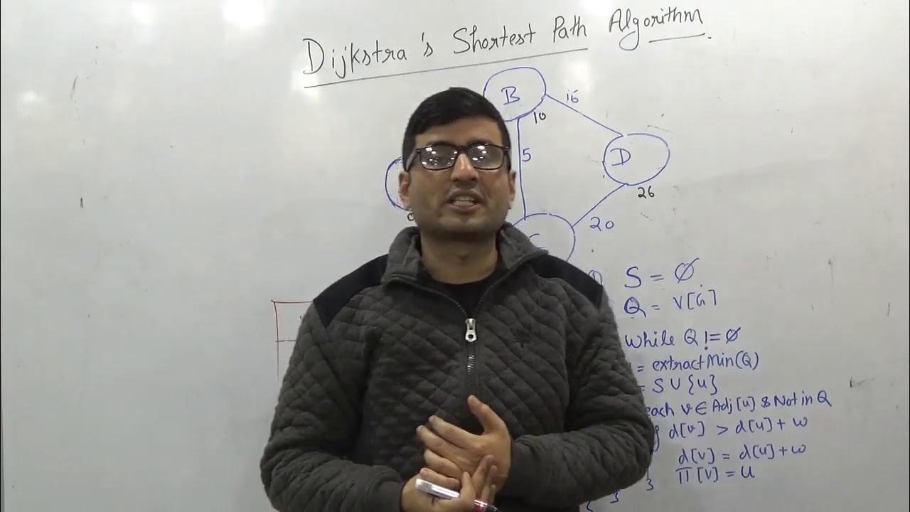
TLDRThis video script discusses the shortest path problem in graphs, specifically focusing on the Dijkstra's algorithm for finding the shortest path from a single origin to all other vertices. It explains the concept of relaxation, the importance of non-negative weights for correct results, and how the algorithm constructs a shortest path tree from the origin. The script also touches on the Bellman-Ford algorithm, which handles negative weights and detects negative cycles, and provides an example to illustrate the algorithm's process.
Takeaways
- 📚 The lecture introduces the problem of finding the shortest path in a graph with a single origin.
- 🛣️ The problem is modeled using a graph where vertices represent cities and edges represent paths between cities, each with a weight.
- 🔢 The weight of an edge could represent the distance or cost to travel, calculated as the sum of the prices of all edges in a path.
- 📈 The shortest path is determined by calculating the weights of all possible paths and finding the minimum.
- 🔄 An important characteristic of shortest paths is the optimal substructure, where any subpath of the shortest path is also the shortest path between its endpoints.
- ⚠️ Negative weight cycles can cause issues in shortest path calculations, as they can lead to infinitely decreasing path weights.
- 🛠️ Two well-known algorithms for solving the single-source shortest path problem are Dijkstra's algorithm and the Bellman-Ford algorithm.
- 🚀 Dijkstra's algorithm assumes all edge weights are non-negative and is efficient for graphs without negative weight cycles.
- 🔄 The Bellman-Ford algorithm can handle graphs with negative weight edges but is more generic and may have a higher processing time.
- 🌳 The result of the shortest path problem is a shortest-path tree rooted at the source vertex, showing the shortest path to all reachable vertices.
- 🔄 The relaxation step in algorithms is crucial for updating the estimated shortest path weights and determining the parent vertices in the shortest-path tree.
Q & A
What is the main topic of the video script?
-The main topic of the video script is the shortest path problem in graphs, focusing on algorithms for finding the shortest path from a single source to all other vertices.
What is the problem modeled in the script?
-The problem modeled in the script is finding the shortest path from Rio de Janeiro to São Paulo, represented as a graph where cities are vertices and the distances between them are edges with weights.
What is the weight of an edge in the context of the script?
-In the context of the script, the weight of an edge represents the distance or cost of the path between two cities.
What is the formula used to calculate the total weight of a path?
-The total weight of a path is calculated as the sum of the weights of all the edges that make up the path.
What is the property of shortest paths that is referred to as the 'greedy property'?
-The 'greedy property' refers to the characteristic that if you have the shortest path from the source to a vertex, any subpath of that path is also the shortest path between the start and end vertices of the subpath.
What happens when there are negative weights in the graph?
-When there are negative weights in the graph, it can lead to a situation where the shortest path cannot be determined if there is a cycle with negative total weight, as passing through the cycle an infinite number of times would result in a path with a weight approaching negative infinity.
What are the two well-known algorithms mentioned in the script for solving the single-source shortest path problem?
-The two well-known algorithms mentioned in the script are Dijkstra's algorithm and Bellman-Ford algorithm.
How does Dijkstra's algorithm handle negative weights?
-Dijkstra's algorithm does not handle negative weights well because it assumes all edge weights are non-negative. It does not account for the possibility of negative cycles that could lead to infinite paths.
What is the data structure used by the Bellman-Ford algorithm to keep track of the shortest paths?
-The Bellman-Ford algorithm uses two sets: one for vertices whose shortest path distance is definitive (known) and one for vertices whose distance is still an estimate (provisional).
What is the result of running the shortest path algorithms in the script?
-The result of running the shortest path algorithms is a shortest path tree rooted at the source vertex, which shows the shortest path to all other reachable vertices.
How does the Bellman-Ford algorithm perform the relaxation step?
-The Bellman-Ford algorithm performs the relaxation step by checking if the current estimate of the shortest path to a vertex can be improved by going through another vertex. If an improvement is found, it updates the estimate and the parent of the vertex in question.
Outlines

This section is available to paid users only. Please upgrade to access this part.
Upgrade NowMindmap

This section is available to paid users only. Please upgrade to access this part.
Upgrade NowKeywords

This section is available to paid users only. Please upgrade to access this part.
Upgrade NowHighlights

This section is available to paid users only. Please upgrade to access this part.
Upgrade NowTranscripts

This section is available to paid users only. Please upgrade to access this part.
Upgrade Now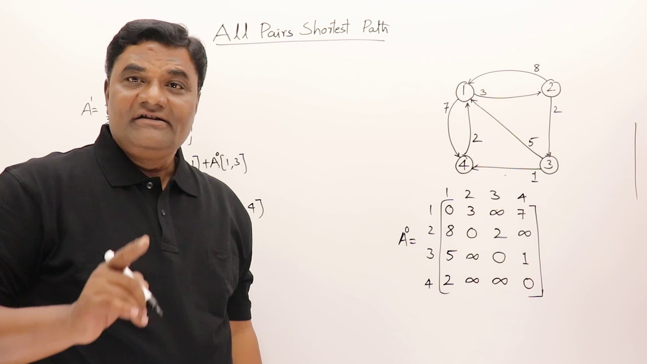


5.0 / 5 (0 votes)