Let's build GPT: from scratch, in code, spelled out.

Summary

本视频介绍了如何使用Transformer架构来训练一个类似于GPT的文本生成模型。通过分析文本序列，模型能够生成连贯的文本。讲解了模型的内部机制，包括自注意力机制、多头注意力、位置编码和前馈网络等关键概念，并展示了如何使用Python和PyTorch实现这些机制。最后，通过在小型数据集上的训练，模型成功生成了类似莎士比亚风格的文本。

Takeaways

• 🤖 介绍了Chachi PT系统，它是一种基于AI的文本交互系统，能够执行文本任务并生成内容。
• 📈 通过比较不同提示生成的结果，展示了Chachi PT是一个概率系统，可以为同一提示提供多种答案。
• 🌐 讨论了Transformer架构的重要性，这是支持Chachi PT和其他类似系统的核心神经网络技术。
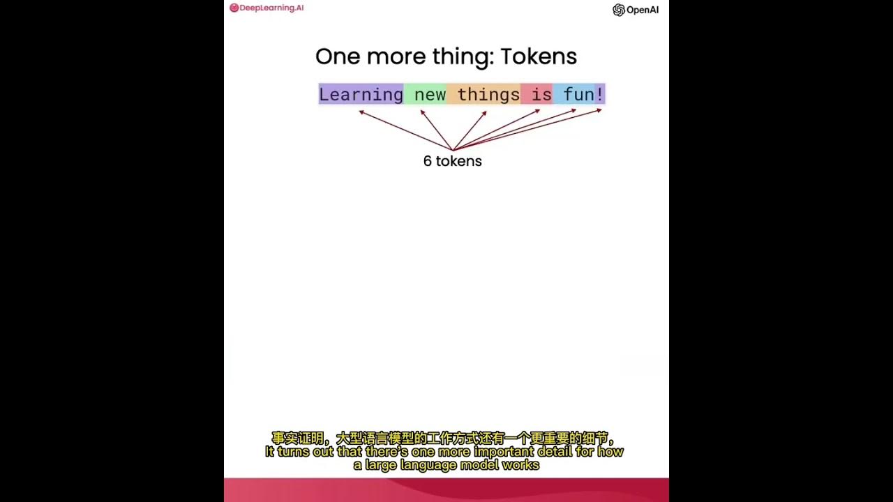
• 📚 提到了使用'tiny Shakespeare'数据集来训练基于字符的Transformer语言模型。
• 🛠️ 强调了训练Transformer模型的过程，包括预训练和微调阶段，以及如何通过迭代和随机采样来训练模型。
• 🔍 解释了如何通过编码器和解码器将文本转换为整数序列，以及如何使用这些序列进行模型训练。
• 📊 展示了如何使用PyTorch库和张量来处理和训练数据，以及如何通过前向和后向传播来训练神经网络。
• 🎯 讨论了模型训练中的损失函数和如何评估模型性能，以及如何通过调整参数来改善模型的训练。
• 🔄 描述了使用自注意力机制（self-attention）来增强模型对文本序列的理解能力。
• 📈 通过实验和结果分析，展示了模型从随机预测到逐渐学习文本模式并生成更合理文本的过程。
• 🚀 最后，提到了如何通过GitHub上的Nano GPT项目来进一步探索和训练Transformer模型。

Q & A

Chachi PT是什么，它如何影响AI社区？

Chachi PT是一种允许用户与AI互动并给予基于文本的任务的系统。它通过生成文本序列来响应用户的提示，从而在AI社区引起了轰动。

如何理解Chachi PT生成的文本是概率性的？

Chachi PT是一个概率性系统，对于同一个提示，它可以生成多个不同的回答。这意味着系统能够根据输入的初始文本序列，预测接下来可能出现的字符或词汇。

Transformer架构是如何在Chachi PT中起作用的？

Transformer架构是Chachi PT的核心，它负责处理序列数据并生成响应。Transformer通过自注意力机制（Self-Attention）和位置编码（Positional Encoding）来理解输入文本的上下文和结构，从而生成连贯和相关的输出文本。

什么是自注意力机制（Self-Attention）？

自注意力机制是Transformer架构中的关键组成部分，它允许模型在处理一个序列时考虑序列中的所有位置，这使得模型能够捕捉到长距离依赖关系。通过自注意力机制，模型可以更好地理解文本中的上下文信息。

为什么Transformer架构在AI领域如此重要？

Transformer架构因其高效的并行处理能力和对长距离依赖关系的捕捉而在AI领域变得极其重要。自从2017年提出以来，它已经被广泛应用于各种AI任务，如机器翻译、文本生成、问答系统等。

如何训练一个基于Transformer的语言模型？

训练一个基于Transformer的语言模型需要大量的文本数据和计算资源。首先，需要对数据进行预处理，如分词、编码和位置编码。然后，通过反向传播和优化算法（如Adam）来调整模型参数，使模型能够根据给定的输入序列生成准确的输出。

在训练Transformer模型时，为什么需要使用位置编码？

位置编码用于给模型提供序列中每个元素的位置信息。由于Transformer架构本身不具备捕捉序列顺序的能力，位置编码通过向输入的每个元素添加一个唯一的位置标记来帮助模型理解元素在序列中的位置。

在训练过程中，为什么需要对模型进行预训练和微调？

预训练是在一个大型的数据集上进行的，目的是让模型学习到语言的通用表示。微调则是在特定任务的数据集上进行的，目的是让模型更好地适应这个任务。通过这两个阶段，模型能够从通用知识中提取出对特定任务有用的信息。

如何评估Chachi PT或类似模型的性能？

模型的性能通常通过损失函数来评估，如交叉熵损失。此外，还可以通过人工评估生成的文本的质量，包括其连贯性、相关性和准确性。在实际应用中，还需要考虑模型的响应时间和计算效率。

在训练Transformer模型时，如何避免过拟合？

为了避免过拟合，可以采用多种技术，如数据增强、正则化、dropout和早停（early stopping）。这些方法可以帮助模型在保持良好性能的同时，避免对训练数据过度敏感。

Outlines

00:00

🤖 介绍Chachi PT和AI交互

本段介绍了Chachi PT系统，这是一个允许与AI交互并给予文本任务的系统。通过示例展示了AI如何根据给定的文本提示生成响应，例如写关于AI重要性的俳句。同时，提到了AI是概率性系统，对于同一个提示可以有多种回答，并且介绍了如何通过Transformer架构来实现这种语言模型。

05:03

📝 训练Transformer基础语言模型

这一部分讨论了如何训练一个基于Transformer的语言模型，特别是字符级别的模型。提到了使用Shakespeare作品作为数据集，并解释了如何将文本字符编码为整数序列。还介绍了如何使用简单的Tokenizer将文本转换为模型可以理解的格式，并展示了如何通过神经网络进行训练。

10:03

🌐 在训练数据中应用Transformer

这一段深入探讨了如何将文本序列或整数序列输入到Transformer中进行训练。详细解释了如何通过随机采样训练集的小片段（chunks）来训练Transformer，并展示了如何构建输入和目标数据集，以及如何通过迭代每个块大小的序列来训练模型。

15:05

🔢 处理批次维度和批量数据

本段讨论了在训练过程中如何处理批次维度和批量数据。解释了如何通过随机偏移量来抓取训练集中的块，并将这些块堆叠成单个张量以进行并行处理。同时，强调了这种处理方式的效率，因为它允许GPU同时处理多个批次数据。

20:06

📈 训练过程中的损失函数和生成函数

这一部分介绍了在训练过程中如何使用损失函数来评估模型的性能，以及如何通过生成函数从模型中生成文本。详细说明了如何计算交叉熵损失，并展示了如何通过softmax函数和负对数似然损失来优化模型。此外，还讨论了如何通过迭代每个块大小的序列来生成文本。

25:07

🔄 实现简单的bigram语言模型

本段展示了如何实现一个简单的bigram语言模型，并通过PyTorch模块直接实现。讨论了如何创建一个嵌入表，并通过嵌入表来预测序列中的下一个字符。同时，介绍了如何通过交叉熵损失来评估模型的质量，并展示了如何通过生成函数来从模型中生成文本。

30:08

🚀 训练和优化模型

这一段讨论了如何使用Adam优化器来训练模型，并通过迭代训练循环来优化模型参数。介绍了如何使用估计损失函数来更准确地衡量训练和验证损失，并展示了如何通过设置模型为评估阶段来提高内存效率。同时，还提到了如何通过简单地增加迭代次数来提高模型性能。

35:09

🎯 理解自注意力机制

本段深入探讨了自注意力机制的数学原理和实现方式。通过一个玩具示例解释了如何使用矩阵乘法来实现有效的加权聚合，并展示了如何通过权重矩阵来控制不同token之间的交互。同时，介绍了如何使用softmax函数来规范化权重，以及如何通过三角形掩码来防止未来信息的流入。

40:12

🛠️ 实现单个自注意力头

这一部分详细介绍了如何实现单个自注意力头，包括如何初始化线性模块来生成查询（Q）、键（K）和值（V）向量。讨论了如何通过点积来计算Q和K之间的相似度，并展示了如何使用softmax函数来获取注意力权重。同时，还介绍了如何通过这些权重来聚合V向量，以及如何通过线性层将聚合结果转换为最终的输出。

45:12

🔄 多头注意力和前馈网络

本段讨论了如何通过并行应用多个自注意力头来实现多头注意力机制，并通过连接它们的输出来增强模型的表达能力。同时，介绍了前馈网络的结构和作用，以及如何将自注意力和前馈网络结合在一起，形成Transformer的基本构建块。此外，还提到了如何通过调整模型的超参数来优化性能。

50:13

📉 优化深度神经网络

这一部分探讨了如何使用残差连接和层归一化来优化深度神经网络。解释了残差连接如何帮助梯度直接从输出传播到输入，从而缓解优化问题。同时，介绍了层归一化如何对每一层的输出进行归一化，以保持模型训练的稳定性。还提到了在模型中实现这些技术的具体方法。

55:14

🔧 调整和扩展Transformer模型

本段讨论了如何通过调整模型的超参数和添加正则化技术（如Dropout）来扩展Transformer模型。介绍了如何通过增加层数、调整嵌入维度和头数来增强模型，并讨论了Dropout如何防止过拟合。同时，展示了如何通过训练更深层次的网络来进一步降低验证损失。

00:15

🎭 从模型中生成文本

这一部分展示了如何使用训练好的Transformer模型来生成文本。讨论了如何通过模型生成大量字符，并将其写入文件。同时，展示了生成文本的示例，虽然这些文本在莎士比亚的风格上是无意义的，但它们在形式上模仿了输入文本文件的结构。

05:18

📚 总结和未来方向

本段总结了如何训练一个解码器型的Transformer模型，并将其与GPT-3进行了比较。讨论了预训练和微调阶段，并指出了如何通过额外的微调步骤将模型从文档完成器转变为问答系统。同时，提到了未来可能的研究方向，包括使用奖励模型和策略梯度优化来进一步优化模型。

Keywords

💡Chachi PT

Chachi PT是一种人工智能系统，它允许用户通过文本任务与AI进行交互。在视频中，Chachi PT被用来生成关于人们理解AI重要性的短诗，展示了AI在生成文本和理解语言模式方面的能力。

💡Transformer架构

Transformer架构是一种深度学习模型，它在自然语言处理领域具有革命性的影响。它通过自注意力机制（Self-Attention）来捕捉输入数据之间的依赖关系，从而在机器翻译等任务中取得了显著的成果。

💡自注意力机制

自注意力机制是一种让神经网络在处理序列数据时能够考虑到序列中不同位置的信息的技术。这种机制使得模型能够捕捉到序列内部的复杂依赖关系，从而提高对语言等序列数据的理解能力。

💡位置编码

位置编码是一种添加到序列数据中的额外信息，用于帮助神经网络理解序列中各个元素的位置。这对于模型正确理解和生成文本至关重要，因为它提供了序列中单词或字符的顺序信息。

💡语言模型

语言模型是一种用于预测和生成自然语言文本的机器学习模型。它通过学习语言的统计规律来理解和生成句子，是自然语言处理领域的基础技术之一。

💡编码器和解码器

在自然语言处理中，编码器和解码器通常是模型的两个主要部分，编码器负责将输入数据转换为内部表示，而解码器则将这些表示转换回输出数据。在Transformer架构中，编码器和解码器通过自注意力机制相互作用，以理解和生成文本。

💡预训练和微调

预训练是指在大规模数据集上训练模型以学习通用知识的过程，而微调则是在特定任务上进一步优化模型性能的过程。预训练使模型掌握语言的基本规律，微调则使模型适应特定的应用场景。

💡多头注意力

多头注意力是一种允许模型在处理信息时考虑多个不同表示子空间的技术。通过并行地学习序列中不同部分的关系，多头注意力可以提高模型对复杂数据的理解能力。

💡层归一化

层归一化是一种在深度神经网络中常用的技术，它通过对每一层的激活值进行归一化处理，来稳定训练过程并加速收敛。这有助于防止梯度消失或爆炸问题，从而提高模型的训练效率。

💡Dropout

Dropout是一种正则化技术，通过在训练过程中随机丢弃（即暂时移除）网络中的一些节点，来防止模型过拟合。这样可以迫使网络学习更加鲁棒的特征，因为它不能依赖于任何一个节点的激活。

Highlights

介绍了Chachi PT系统，它允许与AI交互并完成基于文本的任务。

通过AI生成的俳句来强调人们理解AI的重要性。

展示了ChatGPT的输出，证明了AI是增长的力量，而无知则阻碍我们的进步。

解释了ChatGPT是一个概率系统，对于同一个提示可以给出多种答案。

讨论了Transformer架构，这是ChatGPT背后的核心机制。

提到了2017年的开创性论文《Attention is all you need》，它提出了Transformer架构。

阐述了Transformer神经网络如何通过字符级语言模型来预测文本序列。

介绍了如何使用Python和一些基本的微积分和统计学知识来理解ChatGPT的内部工作原理。

讨论了如何使用GitHub上的Nano GPT存储库来训练Transformer模型。

展示了如何通过字符级Tokenizer将文本转换为整数序列。

解释了如何将整个训练集编码为整数张量，以便输入到Transformer模型中。

讨论了如何将数据集分为训练和验证集，以评估模型的过拟合程度。

介绍了如何使用Transformer模型进行文本序列的训练，包括设置批量大小和块大小。

展示了如何通过简单的bigram语言模型来生成文本，并讨论了其局限性。

讨论了如何使用自注意力机制来改进模型，使模型能够更好地理解和预测文本序列。

介绍了多头注意力的概念，以及如何通过并行处理多个注意力头来提高模型性能。

讨论了位置编码的重要性，以及如何通过位置嵌入来给模型提供关于单词在句子中位置的信息。

提到了如何使用Layer Norm和残差连接来优化深度神经网络的训练。

展示了如何通过训练一个更大的Transformer模型来改进语言生成任务的性能。

Transcripts

hi everyone

so by now you have probably heard of

Chachi PT it has taken the world and the

AI Community by storm and it is a system

that allows you to interact with an AI

and give it text-based tasks so for

example we can ask chatgpt to write us a

small haiku about how important it is

that people understand Ai and then they

can use it to improve the world and make

it more prosperous so when we run this

AI knowledge brings prosperity for all

to see Embrace its power okay not bad

and so you could see that Chachi PT went

from left to right and generated all

these words seek sort of sequentially

now I asked it already the exact same

prompt a little bit earlier and it

generated a slightly different outcome

AI is power to grow ignorance holds us

back learn Prosperity weights

so uh pretty good in both cases and

slightly different so you can see that

chatgpt is a probabilistic system and

for any one prompt it can give us

multiple answers sort of replying to it

now this is just one example of a prompt

people have come up with many many

examples and there are entire websites

that index interactions with charge EBT

and so many of them are quite humorous

explain HTML to me like I'm a dog write

release notes for chess 2. write a note

about Elon Musk buying on Twitter

and so on

so as an example please write a breaking

news article about a leaf falling from a

tree

uh and a shocking turn of events a leaf

has fallen from a treat in the local

park Witnesses report that the leaf

which was previously attached to a

branch of a tree detached itself and

fell to the ground very dramatic so you

can see that this is a pretty remarkable

system and it is what we call a language

model because it it models the sequence

of words or characters or tokens more

generally and it knows how sort of words

follow each other in English language

and so from its perspective what it is

doing is it is completing the sequence

so I give it the start of a sequence and

it completes the sequence with the

outcome and so it's a language model in

that sense

now I would like to focus on the under

the hood of

um under the hood components of what

makes chat GPT work so what is the

neural network under the hood that

models the sequence of these words

and that comes from this paper called

attention is all you need in 2017 a

landmark paper a landmark paper and AI

that produced and proposed the

Transformer architecture

so GPT is short for generally

generatively pre-trained Transformer so

Transformer is the neural nut that

actually does all the heavy lifting

under the hood it comes from this paper

in 2017. now if you read this paper this

reads like a pretty random machine

translation paper and that's because I

think the authors didn't fully

anticipate the impact that the

Transformer would have on the field and

this architecture that they produced in

the context of machine translation in

their case actually ended up taking over

the rest of AI in the next five years

after and so this architecture with

minor changes was copy pasted into a

huge amount of applications in AI in

more recent years and that includes at

the core of chat GPT

now we are not going to what I'd like to

do now is I'd like to build out

something like chatgpt but we're not

going to be able to of course reproduce

chatgpt this is a very serious

production grade system it is trained on

a good chunk of internet and then

there's a lot of pre-training and

fine-tuning stages to it and so it's

very complicated what I'd like to focus

on is just to train a Transformer based

language model and in our case it's

going to be a character level

a language model I still think that is a

very educational with respect to how

these systems work so I don't want to

train on the chunk of Internet we need a

smaller data set in this case I propose

that we work with my favorite toy data

set it's called tiny Shakespeare and

what it is is basically it's a

concatenation of all of the works of

Shakespeare in my understanding and so

this is all of Shakespeare in a single

file this file is about one megabyte

and it's just all of Shakespeare

and what we are going to do now is we're

going to basically model how these

characters follow each other so for

example given a chunk of these

characters like this

are given some context of characters in

the past the Transformer neural network

will look at the characters that I've

highlighted and is going to predict that

g is likely to come next in the sequence

and it's going to do that because we're

going to train that Transformer on

Shakespeare and it's just going to try

to produce uh character sequences that

look like this

and in that process is going to model

all the patterns inside this data so

once we've trained the system I'd just

like to give you a preview we can

generate infinite Shakespeare and of

course it's a fake thing that looks kind

of like Shakespeare

um

apologies for there's some junk that I'm

not able to resolve in in here but

um

you can see how this is going character

by character and it's kind of like

predicting Shakespeare like language so

verily my Lord the sights have left the

again the king coming with my curses

with precious pale and then tronio says

something else Etc and this is just

coming out of the Transformer in a very

similar manner as it would come out in

Chachi PT in our case character by

character in Chachi PT it's coming out

on the token by token level and tokens

are these a sort of like little sub word

pieces so they're not Word level they're

kind of like work chunk level

um and now the I've already written this

entire code to train these Transformers

um and it is in a GitHub repository that

you can find and it's called a nano GPT

so Nano GPT is a repository that you can

find on my GitHub and it's a repository

for training Transformers

um On Any Given text

and what I think is interesting about it

because there's many ways to train

Transformers but this is a very simple

implementation so it's just two files of

300 lines of code each one file defines

the GPT model the Transformer and one

file trains it on some given Text data

set and here I'm showing that if you

train it on a open webtext data set

which is a fairly large data set of web

pages then I reproduce the the

performance of gpt2

so gpt2 is an early version of openai's

GPT from 2017 if I occur correctly and

I've only so far reproduced the the

smallest 124 million parameter model but

basically this is just proving that the

code base is correctly arranged and I'm

able to load the neural network weights

that open AI has released later

so you can take a look at the finished

code here in Nano GPT but what I would

like to do in this lecture is I would

like to basically write this repository

from scratch so we're going to begin

with an empty file and we're going to

define a Transformer piece by piece

we're going to train it on the tiny

Shakespeare data set and we'll see how

we can then generate infinite

Shakespeare and of course this can copy

paste to any arbitrary Text data set

that you like but my goal really here is

to just make you understand and

appreciate how under the hood chat GPT

works and really all that's required is

a Proficiency in Python and some basic

understanding of calculus and statistics

and it would help if you also see my

previous videos on the same YouTube

channel in particular my make more

series where I

Define smaller and simpler neural

network language models so multilevel

perceptrons and so on it really

introduces the language modeling

framework and then here in this video

we're going to focus on the Transformer

neural network itself

okay so I created a new Google collab uh

jupyter notebook here and this will

allow me to later easily share this code

that we're going to develop together

with you so you can follow along so this

will be in the video description later

now here I've just done some

preliminaries I downloaded the data set

the tiny Shakespeare data set at this

URL and you can see that it's about a

one megabyte file

then here I open the input.txt file and

just read in all the text as a string

and we see that we are working with 1

million characters roughly

and the first 1000 characters if we just

print them out are basically what you

would expect this is the first 1000

characters of the tiny Shakespeare data

set roughly up to here

so so far so good next we're going to

take this text and the text is a

sequence of characters in Python so when

I call the set Constructor on it I'm

just going to get the set of all the

characters that occur in this text

and then I call list on that to create a

list of those characters instead of just

a set so that I have an ordering an

arbitrary ordering

and then I sort that

so basically we get just all the

characters that occur in the entire data

set and they're sorted now the number of

them is going to be our vocabulary size

these are the possible elements of our

sequences and we see that when I print

here the characters

there's 65 of them in total there's a

space character and then all kinds of

special characters

and then capitals and lowercase letters

so that's our vocabulary and that's the

sort of like possible characters that

the model can see or emit

okay so next we would like to develop

some strategy to tokenize the input text

now when people say tokenize they mean

convert the raw text as a string to some

sequence of integers According to some

notebook According to some vocabulary of

possible elements

so as an example here we are going to be

building a character level language

model so we're simply going to be

translating individual characters into

integers

so let me show you a chunk of code that

sort of does that for us

so we're building both the encoder and

the decoder and let me just talk through

What's Happening Here

when we encode an arbitrary text like hi

there we're going to receive a list of

integers that represents that string so

for example 46 47 Etc

and then we also have the reverse

mapping so we can take this list and

decode it to get back the exact same

string

so it's really just like a translation

two integers and back for arbitrary

string and for us it is done on a

character level

now the way this was achieved is we just

iterate over all the characters here and

create a lookup table from the character

to the integer and vice versa and then

to encode some string we simply

translate all the characters

individually and to decode it back we

use the reverse mapping and concatenate

all of it

now this is only one of many possible

encodings or many possible sort of

tokenizers and it's a very simple one

but there's many other schemas that

people have come up with in practice so

for example Google uses a sentence piece

uh so sentence piece will also encode

text into integers but in a different

schema and using a different vocabulary

and sentence piece is a sub word sort of

tokenizer and what that means is that

you're not encoding entire words but

you're not also encoding individual

characters it's it's a sub word unit

level and that's usually what's adopted

in practice for example also openai has

this Library called tick token that uses

a pipe pair encoding tokenizer

um and that's what GPT uses

and you can also just encode words into

like hello world into a list of integers

so as an example I'm using the tick

token Library here

I'm getting the encoding for gpt2 or

that was used for gpt2

instead of just having 65 possible

characters or tokens they have 50 000

tokens

and so when they encode the exact same

string High there we only get a list of

three integers but those integers are

not between 0 and 64. they are between 0

and 5000 50 256.

so basically you can trade off the code

book size and the sequence lengths so

you can have a very long sequences of

integers with very small vocabularies or

you can have a short

um

sequences of integers with very large

vocabularies and so typically people use

in practice the sub word encodings but

I'd like to keep our tokenizer very

simple so we're using character level

tokenizer

and that means that we have very small

code books we have very simple encode

and decode functions but we do get very

long sequences as a result but that's

the level at which we're going to stick

with this lecture because it's the

simplest thing okay so now that we have

an encoder and a decoder effectively a

tokenizer we can tokenize the entire

training set of Shakespeare so here's a

chunk of code that does that

and I'm going to start to use the

pytorch library and specifically the

torch.tensor from the pytorch library

so we're going to take all of the text

in tiny Shakespeare encode it and then

wrap it into a torch.tensor to get the

data tensor so here's what the data

tensor looks like when I look at just

the first 1000 characters or the 1000

elements of it

so we see that we have a massive

sequence of integers and this sequence

of integers here is basically an

identical translation of the first 1000

characters here

so I believe for example that zero is a

new line character and maybe one is a

space not 100 sure but from now on the

entire data set of text is

re-represented as just it just stretched

out as a single very large uh sequence

of integers

let me do one more thing before we move

on here I'd like to separate out our

data set into a train and a validation

split so in particular we're going to

take the first 90 of the data set and

consider that to be the training data

for the Transformer and we're going to

withhold the last 10 percent at the end

of it to be the validation data and this

will help us understand to what extent

our model is overfitting so we're going

to basically hide and keep the

validation data on the side because we

don't want just a perfect memorization

of this exact Shakespeare we want a

neural network that sort of creates

Shakespeare like text and so it should

be fairly likely for it to produce

the actual like stowed away uh true

Shakespeare text

um and so we're going to use this to get

a sense of the overfitting okay so now

we would like to start plugging these

text sequences or integer sequences into

the Transformer so that it can train and

learn those patterns

now the important thing to realize is

we're never going to actually feed the

entire text into Transformer all at once

that would be computationally very

expensive and prohibitive so when we

actually train a Transformer on a lot of

these data sets we only work with chunks

of the data set and when we train the

Transformer we basically sample random

little chunks out of the training set

and train them just chunks at a time and

these chunks have basically some kind of

a length

and as a maximum length now the maximum

length typically at least in the code I

usually write is called block size

you can you can find it on the different

names like context length or something

like that let's start with the block

size of just eight and let me look at

the first train data characters the

first block size plus one characters

I'll explain why plus one in a second

so this is the first nine characters in

the sequence in the training set

now what I'd like to point out is that

when you sample a chunk of data like

this so say that these nine characters

out of the training set

this actually has multiple examples

packed into it

and that's because all of these

characters follow each other

and so what this thing is going to say

when we plug it into a Transformer is

we're going to actually simultaneously

train it to make prediction at every one

of these positions

now in the in a chunk of nine characters

there's actually eight individual

examples packed in there

so there's the example that one 18 when

in the context of 18 47 likely comes

next in the context of 18 and 47 56

comes next in the context of 1847-56 57

can come next and so on so that's the

eight individual examples let me

actually spell it out with code

so here's a chunk of code to illustrate

X are the inputs to the Transformer it

will just be the first block size

characters

y will be the next block size characters

so it's offset by one

and that's because y are the targets for

each position in the input

and then here I'm iterating over all the

block size of 8. and the context is

always all the characters in X up to T

and including t

and the target is always the teeth

character but in the targets array why

so let me just run this

and basically it spells out what I've

said in words these are the eight

examples hidden in a chunk of nine

characters that we uh sampled from the

training set

I want to mention one more thing we

train on all the eight examples here

with context between one all the way up

to context of block size

and we train on that not just for

computational reasons because we happen

to have the sequence already or

something like that it's not just done

for efficiency it's also done to make

the Transformer Network be used to

seeing contexts all the way from as

little as one all the way to block size

and we'd like the transform to be used

to seeing everything in between and

that's going to be useful later during

inference because while we're sampling

we can start the sampling generation

with as little as one character of

context and the Transformer knows how to

predict the next character with all the

way up to just one context of one and so

then it can predict everything up to

block size and after block size we have

to start truncating because the

Transformer will never receive more than

block size inputs when it's predicting

the next character

Okay so we've looked at the time

dimension of the tensors that are going

to be feeding into the Transformer

there's one more Dimension to care about

and that is the batch dimension and so

as we're sampling these chunks of text

we're going to be actually every time

we're going to feed them into a

Transformer we're going to have many

batches of multiple chunks of text that

are all like stacked up in a single

tensor and that's just done for

efficiency just so that we can keep the

gpus busy because they are very good at

parallel processing of

um of data and so we just want to

process multiple chunks all at the same

time but those chunks are processed

completely independently they don't talk

to each other and so on so let me

basically just generalize this and

introduce a batch Dimension here's a

chunk of code

let me just run it and then I'm going to

explain what it does

so here because we're going to start

sampling random locations in the data

set to pull chunks from I am setting the

seed so that

um in the random number generator so

that the numbers I see here are going to

be the same numbers you see later if you

try to reproduce this

now the back size here is how many

independent sequences we are processing

every forward backward pass of the

Transformer

the block size as I explained is the

maximum context length to make those

predictions

so let's say by size 4 block size 8 and

then here's how we get batch

for any arbitrary split if the split is

a training split then we're going to

look at train data otherwise and

validata

that gets us the data array and then

when I Generate random positions to grab

a chunk out of

I actually grab I actually generate

batch size number of

random offsets

so because this is four we are IX is

going to be a four numbers that are

randomly generated between 0 and Len of

data minus block size so it's just

random offsets into the training set

and then X's as I explained are the

first block size characters starting at

I

the Y's are the offset by one of that so

just add plus one

and then we're going to get those chunks

for every one of integers I in IX and

use a torch.stack to take all those

one-dimensional tensors as we saw here

and we're going to

um stack them up at rows

and so they all become a row in a four

by eight tensor

so here's where I'm printing then

when I sample a batch XP and YB

the input the Transformer now are

the input X is the four by eight tensor

four uh rows of eight columns

and each one of these is a chunk of the

training set

and then the targets here are in the

associated array Y and they will come in

through the Transformer all the way at

the end to create the loss function so

they will give us the correct answer for

every single position inside X

and then these are the four independent

rows

so spelled out as we did before

this four by eight array contains a

total of 32 examples and they're

completely independent as far as the

Transformer is concerned

uh so when the

input is 24 the target is 43 or rather

43 here in the Y array when the input is

2443 the target is 58.

when the input is 24 43.58 the target is

5 Etc or like when it is a 5258 one the

target is 58.

right so you can sort of see this

spelled out these are the 32 independent

examples packed in to a single batch of

the input X and then the desired targets

are in y

and so now this integer tensor of X is

going to feed into the Transformer

and that Transformer is going to

simultaneously process all these

examples and then look up the correct

um integers to predict in every one of

these positions in the tensor y okay so

now that we have our batch of input that

we'd like to feed into a Transformer

let's start basically feeding this into

neural networks now we're going to start

off with the simplest possible neural

network which in the case of language

modeling in my opinion is the bigram

language model and we've covered the

background language model in my make

more series in a lot of depth and so

here I'm going to sort of go faster and

let's just implement the pytorch module

directly that implements the bigram

language model

so I'm importing the pytorch and then

module

uh for reproducibility

and then here I'm constructing a diagram

language model which is a subclass of NN

module

and then I'm calling it and I'm passing

in the inputs and the targets

and I'm just printing now when the

inputs and targets come here you see

that I'm just taking the index the

inputs X here which I rename to idx and

I'm just passing them into this token

embedding table

so what's going on here is that here in

the Constructor

we are creating a token embedding table

and it is of size vocab size by vocab

size

and we're using nn.embedding which is a

very thin wrapper around basically a

tensor of shape both capsized by vocab

size

and what's happening here is that when

we pass idx here every single integer in

our input is going to refer to this

embedding table and is going to pluck

out a row of that embedding table

corresponding to its index so 24 here

we'll go to the embedding table and

we'll pluck out the 24th row and then 43

will go here and block out the 43rd row

Etc and then Pi torch is going to

arrange all of this into a batch by Time

by Channel tensor in this case batch is

4 time is 8 and C which is the channels

is vocab size or 65. and so we're just

going to pluck out all those rows

arrange them in a b by T by C and now

we're going to interpret this as the

logits which are basically the scores

for the next character in the sequence

and so what's happening here is we are

predicting what comes next based on just

the individual identity of a single

token and you can do that because

um I mean currently the tokens are not

talking to each other and they're not

seeing any context except for they're

just seeing themselves so I'm a I'm a

token number five and then I can

actually make pretty decent predictions

about what comes next just by knowing

that I'm token five because some

characters know cert follow other

characters in in typical scenarios so we

saw a lot of this in a lot more depth in

the make more series and here if I just

run this then we currently get the

predictions the scores the logits for

every one of the four by eight positions

now that we've made predictions about

what comes next we'd like to evaluate

the loss function and so in make more

series we saw that a good way to measure

a loss or like a quality of the

predictions is to use the negative log

likelihood loss which is also

implemented in pytorch under the name

cross entropy

so what we'd like to do here is

loss is the cross entropy on the

predictions and the targets and so this

measures the quality of the logits with

respect to the Targets in other words we

have the identity of the next character

so how well are we predicting the next

character based on Illusions and

intuitively the correct

um the correct dimension of logits uh

depending on whatever the target is

should have a very high number and all

the other dimensions should be very low

number right

now the issue is that this won't

actually this is what we want we want to

basically output the logits and the loss

this is what we want but unfortunately

uh this won't actually run

we get an error message but intuitively

we want to measure this now when we go

to the pi torch cross entropy

a documentation here

um

we're trying to call the cross entropy

in its functional form so that means we

don't have to create like a module for

it

but here when we go to the documentation

you have to look into the details of how

pytorch expects these inputs and

basically the issue here is by torch

expects if you have multi-dimensional

input which we do because we have a b by

T by C tensor then it actually really

wants the channels to be the second

dimension here

so if you um so basically it wants a b

by C by T instead of a b by T by C

and so it's just the details of how

pytorch treats

um these kinds of inputs and so we don't

actually want to deal with that so what

we're going to do instead is we need to

basically reshape our logits so here's

what I like to do I like to take

basically give names to the dimensions

so launches.shape is B by T by C and

unpack those numbers

and then let's say that logits equals

logits.view

and we want it to be a b times c b times

T by C so just a two-dimensional array

right so we're going to take all the

we're going to take all of these

um

positions here and we're going to uh

stretch them out in a one-dimensional

sequence

and preserve the channel Dimension as

the second dimension

so we're just kind of like stretching

out the array so it's two-dimensional

and in that case it's going to better

conform to what pi torch sort of expects

in its dimensions

now we have to do the same to targets

because currently targets

are of shape B by T and we want it to be

just B times T so one dimensional now

alternatively you could always still

just do -1 because Pi torch will guess

what this should be if you want to lay

it out but let me just be explicit on

say Q times t

once we've reshaped this it will match

the cross entropy case

and then we should be able to evaluate

our loss

okay so with that right now and we can

do loss and So currently we see that the

loss is 4.87

now because our we have 65 possible

vocabulary elements we can actually

guess at what the loss should be and in

particular

we covered negative log likelihood in a

lot of detail we are expecting log or

long of

um 1 over 65 and negative of that

so we're expecting the loss to be about

4.1217 but we're getting 4.87 and so

that's telling us that the initial

predictions are not super diffuse

they've got a little bit of entropy and

so we're guessing wrong

uh so uh yes but actually we're I able

we are able to evaluate the loss okay so

now that we can evaluate the quality of

the model on some data we'd likely also

be able to generate from the model so

let's do the generation now I'm going to

go again a little bit faster here

because I covered all this already in

previous videos

so

here's a generate function for the model

so we take some uh we take the the same

kind of input idx here

and basically

this is the current context of some

characters in a batch in some batch

so it's also B by T and the job of

generate is to basically take this B by

T and extend it to be B by T plus one

plus two plus three and so it's just

basically it contains the generation in

all the batch dimensions in the time

dimension

So that's its job and we'll do that for

Max new tokens

so you can see here on the bottom

there's going to be some stuff here but

on the bottom whatever is predicted is

concatenated on top of the previous idx

along the First Dimension which is the

time Dimension to create a b by T plus

one

so that becomes the new idx so the job

of generators to take a b by T and make

it a b by T plus one plus two plus three

as many as we want maximum tokens so

this is the generation from the model

now inside the generation what we're

what are we doing we're taking the

current indices we're getting the

predictions so we get those are in the

logits

and then the loss here is going to be

ignored because

um we're not we're not using that and we

have no targets that are sort of ground

truth targets that we're going to be

comparing with

then once we get the logits we are only

focusing on the last step so instead of

a b by T by C we're going to pluck out

the negative one the last element in the

time dimension

because those are the predictions for

what comes next

so that this is the logits which we then

convert to probabilities via softmax and

then we use torch that multinomial to

sample from those probabilities and we

ask by torch to give us one sample

and so idx next will become a b by one

because in each one of the batch

Dimensions we're going to have a single

prediction for what comes next so this

num samples equals one will make this be

a one

and then we're going to take those

integers that come from the sampling

process according to the probability

distribution given here

and those integers got just concatenated

on top of the current sort of like

running stream of integers and this

gives us a p by T plus one

and then we can return that now one

thing here is you see how I'm calling

self of idx which will end up going to

the forward function I'm not providing

any Targets So currently this would give

an error because targets is uh is uh

sort of like not given so target has to

be optional so targets is none by

default and then if targets is none then

there's no loss to create so it's just

loss is none but else all of this

happens and we can create a loss

so this will make it so

um

if we have the targets we provide them

and get a loss if we have no targets

we'll just get the logits

so this here will generate from the

model

um and let's take that for a ride now

oops

so I have another code chunk here which

will generate for the model from the

model and okay this is kind of crazy so

maybe let me let me break this down

so these are the idx right

I'm creating a batch will be just one

time will be just one

so I'm creating a little one by one

tensor and it's holding a zero

and the D type the data type is integer

so 0 is going to be how we kick off the

generation and remember that zero is uh

is the element standing for a new line

character so it's kind of like a

reasonable thing to to feed in as the

very first character in a sequence to be

the new line

um so it's going to be idx which we're

going to feed in here then we're going

to ask for 100 tokens

and then enter generate will continue

that

now because uh generate works on the

level of batches we then have to index

into the zero throw to basically unplug

the um

the single bash Dimension that exists

and then that gives us a um

time steps it's just a one-dimensional

array of all the indices which we will

convert to simple python list

from pytorch tensor so that that can

feed into our decode function and

convert those integers into text

so let me bring this back and we're

generating 100 tokens let's run

and uh here's the generation that we

achieved so obviously it's garbage and

the reason it's garbage is because this

is a totally random model so next up

we're going to want to train this model

now one more thing I wanted to point out

here is

this function is written to be General

but it's kind of like ridiculous right

now because

we're feeding in all this we're building

out this context and we're concatenating

it all and we're always feeding it all

into the model

but that's kind of ridiculous because

this is just a simple background model

so to make for example this prediction

about K we only needed this W but

actually what we fed into the model is

we fed the entire sequence and then we

only looked at the very last piece and

predicted k

so the only reason I'm writing it in

this way is because right now this is a

bygram model but I'd like to keep this

function fixed and I'd like it to work

later when our character is actually

basically look further in the history

and so right now the history is not used

so this looks silly but eventually the

history will be used and so that's why

we want to do it this way so just a

quick comment on that so now we see that

this is um random so let's train the

model so it becomes a bit less random

okay let's Now train the model so first

what I'm going to do is I'm going to

create a pytorch optimization object

so here we are using the optimizer

atom W

now in the make more series we've only

ever used stochastic gradient descent

the simplest possible Optimizer which

you can get using the SGD instead but I

want to use Adam which is a much more

advanced and popular Optimizer and it

works extremely well for a typical good

setting for the learning rate is roughly

3E negative four but for very very small

networks luck is the case here you can

get away with much much higher learning

rates running negative three or even

higher probably

but let me create the optimizer object

which will basically take the gradients

and update the parameters using the

gradients

and then here

our batch size up above was only four so

let me actually use something bigger

let's say 32 and then for some number of

steps

um we are sampling a new batch of data

we're evaluating the loss we're zeroing

out all the gradients from the previous

step getting the gradients for all the

parameters and then using those

gradients to update our parameters so

typical training loop as we saw in the

make more series

so let me now uh run this

for say 100 iterations and let's see

what kind of losses we're gonna get

so we started around 4.7

and now we're going to down to like 4.6

4.5

Etc so the optimization is definitely

happening but

um let's uh sort of try to increase the

number of iterations and only print at

the end

because we probably will not train for

longer

okay so we're down to 3.6 roughly

roughly down to three

this is the most janky optimization

okay it's working let's just do ten

thousand

and then from here we want to copy this

and hopefully we're going to get

something reasonable and of course it's

not going to be Shakespeare from a

background model but at least we see

that the loss is improving and hopefully

we're expecting something a bit more

reasonable

okay so we're down there about 2.5 ish

let's see what we get

okay

dramatic improvements certainly on what

we had here

so let me just increase the number of

tokens

okay so we see that we're starting to

get something at least like

reasonable ish

um

certainly not Shakespeare but the model

is making progress so that is the

simplest possible model

so now what I'd like to do is

obviously that this is a very simple

model because the tokens are not talking

to each other so given the previous

context of whatever was generated we're

only looking at the very last character

to make the predictions about what comes

next so now these uh now these tokens

have to start talking to each other and

figuring out what is in the context so

that they can make better predictions

for what comes next and this is how

we're going to kick off the Transformer

okay so next I took the code that we

developed in this Jupiter notebook and I

converted it to be a script and I'm

doing this because I just want to

simplify our intermediate work into just

the final product that we have at this

point

so in the top here I put all the hyper

parameters that we've defined I

introduced a few and I'm going to speak

to that in a little bit otherwise a lot

of this should be recognizable

reproducibility

read data get the encoder in the decoder

create the training test splits I use

the uh kind of like data loader that

gets a batch of the inputs and targets

this is new and I'll talk about it in a

second

now this is the background language

model that we developed and it can

forward and give us a logits and loss

and it can generate

and then here we are creating the

optimizer and this is the training Loop

so everything here should look pretty

familiar now some of the small things

that I added number one I added the

ability to run on a GPU if you have it

so if you have a GPU then you can this

will use Cuda instead of just CPU and

everything will be a lot more faster now

when device becomes screwed up then we

need to make sure that when we load the

data we move it to device

when we create the model we want to move

the model parameters to device

so as an example here we have the NN

embedding table and it's got a double

weight inside it which stores the sort

of lookup table so that would be moved

to the GPU so that all the calculations

here happen on the GPU and they can be a

lot faster

and then finally here when I'm creating

the context that feeds into generate I

have to make sure that I create on the

device

number two what I introduced is

the fact that here in the training Loop

here I was just printing the Lost dot

item

inside the training Loop but this is a

very noisy measurement of the current

loss because every batch will be more or

less lucky

and so what I want to do usually is I

have an estimate loss function and the

estimated loss basically then goes up

here

and it averages up the loss over

multiple batches

so in particular we're going to iterate

invalider times and we're going to

basically get our loss and then we're

going to get the average loss for both

splits and so this will be a lot less

noisy

so here what we call the estimate loss

we're going to report the pretty

accurate train and validation loss

now when we come back up you'll notice a

few things here I'm setting the model to

evaluation phase and down here I'm

resetting it back to training phase

now right now for our model as is this

this doesn't actually do anything

because the only thing inside this model

is this nn.embedding and

um this this network would behave both

would be have the same in both

evaluation mode and training mode we

have no Dropout layers we have no

bathroom layers Etc but it is a good

practice to Think Through what mode your

neural network is in because some layers

will have different Behavior at

inference time or training time

and

there's also this context manager

torch.nograd and this is just telling

pytorch that everything that happens

inside this function we will not call

that backward on and so Patrick can be a

lot more efficient with its memory use

because it doesn't have to store all the

intermediate variables because we're

never going to call backward and so it

can it can be a lot more memory

efficient in that way so also a good

practice to tell Pi torch when we don't

intend to do back propagation

so right now the script is about 120

lines of code of and that's kind of our

starter code

I'm calling it background.pi and I'm

going to release it later now running

this script gives us output in the

terminal and it looks something like

this

it basically as I ran this code it was

giving me the train loss and Val loss

and we see that we convert to somewhere

around 2.5

with the migrant model and then here's

the sample that we produced at the end

and so we have everything packaged up in

the script and we're in a good position

now to iterate on this okay so we are

almost ready to start writing our very

first self-attention block for

processing these tokens

now before we actually get there I want

to get you used to a mathematical trick

that is used in the self attention

inside a Transformer and is really just

like at the heart of an efficient

implementation of self-attention and so

I want to work with this toy example you

just get used to this operation and then

it's going to make it much more clear

once we actually get to um to it in the

script again

so let's create a b by T by C where B T

and C are just 4 8 and 2 in the story

example and these are basically channels

and we have batches and we have the time

component and we have some information

at each point in the sequence so C

now what we would like to do is we would

like these um tokens so we have up to

eight tokens here in a batch and these

eight tokens are currently not talking

to each other and we would like them to

talk to each other we'd like to couple

them

and in particular we don't we we want to

couple them in a very specific way so

the token for example at the fifth

location it should not communicate with

tokens in the sixth seventh and eighth

location

because those are future tokens in the

sequence

the token on the fifth location should

only talk to the one in the fourth third

second and first

so it's only so information only flows

from previous context to the current

timestamp and we cannot get any

information from the future because we

are about to try to predict the future

so

what is the easiest way for tokens to

communicate okay the easiest way I would

say is okay if we are up to if we're a

fifth token and I'd like to communicate

with my past the simplest way we can do

that is to just do a weight is to just

do an average of all the um of all the

preceding elements so for example if I'm

the fifth token I would like to take the

channels that make up that are

information at my step but then also the

channels from the four step third step

second step in the first step I'd like

to average those up and then that would

become sort of like a feature Vector

that summarizes me in the context of my

history

now of course just doing a sum or like

an average is an extremely weak form of

interaction like this communication is

extremely lossy we've lost a ton of

information about the spatial

Arrangements of all those tokens but

that's okay for now we'll see how we can

bring that information back later

for now what we would like to do is

for every single batch element

independently

for every teeth token in that sequence

we'd like to now calculate the average

of all the vectors in all the previous

tokens and also at this token

so let's write that out

um I have a small snippet here and

instead of just fumbling around let me

just copy paste it and talk to it

so in other words we're going to create

X

and bow is short for backup words

because backup words is um is kind of

like um

a term that people use when you are just

averaging up things so it's just a bag

of words basically there's a word stored

on every one of these eight locations

and we're doing a bag of words such as

averaging

so in the beginning we're going to say

that it's just initialized at Zero and

then I'm doing a for Loop here so we're

not being efficient yet that's coming

but for now we're just iterating over

all the batch Dimensions independently

iterating over time

and then the previous tokens are at this

batch Dimension and then everything up

to and including the teeth token okay

so when we slice out X in this way xrev

Becomes of shape

um how many T elements there were in the

past and then of course C so all the two

dimensional information from these log

tokens

so that's the previous sort of chunk of

um tokens from my current sequence

and then I'm just doing the average or

the mean over the zeroth dimension so

I'm averaging out the time here

and I'm just going to get a little C

one-dimensional Vector which I'm going

to store in X background words

so I can run this and uh this is not

going to be very informative because

let's see so this is x sub 0. so this is

the zeroth batch element and then expo

at zero now

you see how the at the first location

here you see that the two are equal and

that's because it's we're just doing an

average of this one token

but here this one is now an average of

these two

and now this one is an average of these

three

and so on

so uh and this last one is the average

of all of these elements so vertical

average just averaging up all the tokens

now gives this outcome here

so this is all well and good but this is

very inefficient now the trick is that

we can be very very efficient about

doing this using matrix multiplication

so that's the mathematical trick and let

me show you what I mean let's work with

the toy example here

let me run it and I'll explain

I have a simple Matrix here that is a

three by three of all ones

a matrix B of just random numbers and

it's a three by two

and a matrix C which will be three by

three multiply three by two which will

give out a three by two

so here we're just using

um

matrix multiplication

so a multiply B gives us C

okay so how are these numbers in C

achieved right so this number in the top

left is the first row of a DOT product

with the First Column of B

and since all the the row of a right now

is all just once

then the dot product here with with this

column of B is just going to do a sum of

these of this column so 2 plus 6 plus 6

is 14.

the element here and the output of C is

also the first column here the first row

of a multiplied now with the second

column of B so 7 plus 4 plus plus 5 is

16.

now you see that there's repeating

elements here so this 14 again is

because this row is again all once and

it's multiplying the First Column of B

so we get 14. and this one is and so on

so this last number here is the last row

dot product last column

now the trick here is uh the following

this is just a boring number of

um it's just a boring array of all ones

but torch has this function called trell

which is short for a triangular

uh something like that and you can wrap

it in torched at once and it will just

return the lower triangular portion of

this

okay

so now it will basically zero out uh

these guys here so we just get the lower

triangular part well what happens if we

do that

so now we'll have a like this and B like

this and now what are we getting here in

C

well what is this number well this is

the first row times the First Column and

because this is zeros

uh these elements here are now ignored

so we just get a two

and then this number here is the first

row times the second column and because

these are zeros they get ignored and

it's just seven the seven multiplies

this one

but look what happened here because this

is one and then zeros we what ended up

happening is we're just plucking out the

row of this row of B and that's what we

got

now here we have 1 1 0. so here one one

zero dot product with these two columns

will now give us two plus six which is

eight and seven plus four which is 11.

and because this is one one one we ended

up with the addition of all of them

and so basically depending on how many

ones and zeros we have here we are

basically doing a sum currently of a

variable number of these rows and that

gets deposited into C

So currently we're doing sums because

these are ones but we can also do

average right and you can start to see

how we could do average of the rows of B

uh sort of in an incremental fashion

because we don't have to we can

basically normalize these rows so that

they sum to one and then we're going to

get an average

so if we took a and then we did a equals

a divide a torch.sum

in the um

of a in the warmth

Dimension and then let's keep them as

true so therefore the broadcasting will

work out

so if I rerun this you see now that

these rows now sum to one so this row is

one this row is 0.5.50 and here we get

one thirds

and now when we do a multiply B what are

we getting

here we are just getting the first row

first row

here now we are getting the average of

the first two rows

okay so 2 and 6 average is four and four

and seven average is 5.5

and on the bottom here we are now

getting the average of these three rows

so the average of all of elements of B

are now deposited here

and so you can see that by manipulating

these uh elements of this multiplying

Matrix and then multiplying it with any

given Matrix we can do these averages in

this incremental fashion because we just

get

um

and we can manipulate that based on the

elements of a okay so that's very

convenient so let's swing back up here

and see how we can vectorize this and

make it much more efficient using what

we've learned

so in particular

we are going to produce an array a but

here I'm going to call it way short for

weights

but this is r a

and this is how much of every row we

want to average up and it's going to be

an average because you can see it in

these rows sum to 1.

so this is our a and then our B in this

example of course is

X

so it's going to happen here now is that

we are going to have an expo 2.

and this Expo 2 is going to be way

multiplying

RX

so let's think this through way is T by

T and this is Matrix multiplying in pi

torch a b by T by C

and it's giving us

uh the what shape so pytorch will come

here and then we'll see that these

shapes are not the same so it will

create a batch Dimension here and this

is a batched matrix multiply

and so it will apply this matrix

multiplication in all the batch elements

in parallel

and individually and then for each batch

element there will be a t by T

multiplying T by C exactly as we had

below

so this will now create

B by T by C

and X both 2 will now become identical

to Expo

so

we can see that torch.all close

of Expo and Expo 2 should be true now

so this kind of like misses us that uh

these are in fact the same

so Expo and Expo 2 if I just print them

uh okay we're not going to be able to

okay we're not going to be able to just

stare it down but

um

well let me try Expo basically just at

the zeroth element and Expo two at the

zeroth element so just the first batch

and we should see that this and that

should be identical which they are

right so what happened here the trick is

we were able to use batched Matrix

multiply

to do this uh aggregation really and

it's awaited aggregation and the weights

are specified in this T by T array

and we're basically doing weighted sums

and uh these weighted sums are according

to the weights inside here they take on

sort of this triangular form

and so that means that a token at the

teeth Dimension will only get uh sort of

um information from the um tokens

preceding it so that's exactly what we

want and finally I would like to rewrite

it in one more way

and we're going to see why that's useful

so this is the third version and it's

also identical to the first and second

but let me talk through it it uses

softmax

so

Trill here is this Matrix lower

triangular ones

way begins as all zero

okay so if I just print way in the

beginning it's all zero

then I used

masked fill

so what this is doing is

wait that masked fill it's all zeros and

I'm saying for all the elements where

Trill is equals equals zero make them be

negative Infinity

so all the elements where Trill is zero

will become negative Infinity now

so this is what we get

and then the final one here is softmax

so if I take a soft Max along every

single so dim is negative one so along

every single row

if I do a soft Max what is that going to

do

well softmax is um

it's also like a normalization operation

right

and so spoiler alert you get the exact

same Matrix

let me bring back the softmax

and recall that in softmax we're going

to exponentiate every single one of

these

and then we're going to divide by the

sum

and so for if we exponentiate every

single element here we're going to get a

one and here we're going to get uh

basically zero zero zero zero zero

everywhere else

and then when we normalize we just get

one here we're going to get 1 1 and then

zeros and then softmax will again divide

and this will give us 0.5.5 and so on

and so this is also the uh the same way

to produce this mask

now the reason that this is a bit more

interesting and the reason we're going

to end up using it and solve a tension

is that

these weights here begin uh with zero

and you can think of this as like an

interaction strength or like an affinity

so basically it's telling us how much of

each token from the past do we want to

Aggregate and average up

and then this line is saying tokens from

the past cannot communicate by setting

them to negative Infinity we're saying

that we will not aggregate anything from

those tokens

and so basically this then goes through

softmax and through the weighted and

this is the aggregation through matrix

multiplication

and so what this is now is you can think

of these as

um these zeros are currently just set by

us to be zero but a quick preview is

that these affinities between the tokens

are not going to be just constant at

zero they're going to be data dependent

these tokens are going to start looking

at each other and some tokens will find

other tokens more or less interesting

and depending on what their values are

they're going to find each other

interesting to different amounts and I'm

going to call those affinities I think

and then here we are saying the future

cannot communicate with the past we're

going to clamp them

and then when we normalize and sum we're

going to aggregate sort of their values

depending on how interesting they find

each other

and so that's the preview for

self-attention and basically long story

short from this entire section is that

you can do weighted aggregations of your

past elements

by having by using matrix multiplication

of a lower triangular fashion

and then the elements here in the lower

triangular part are telling you how much

of each element fuses into this position

so we're going to use this trick now to

develop the self-attention block so

first let's get some quick preliminaries

out of the way

first the thing I'm kind of bothered by

is that you see how we're passing in

vocab size into the Constructor there's

no need to do that because vocab size

has already defined up top as a global

variable so there's no need to pass this

stuff around

next one I want to do is I don't want to

actually create I want to create like a

level of interaction here where we don't

directly go to the embedding for the um

logits but instead we go through this

intermediate phase because we're going

to start making that bigger so let me

introduce a new variable and embed a

short for a number of embedding

dimensions

so an embed

here

will be say 32. that was a suggestion

from GitHub by the way it also showed us

to 32 which is a good number

so this is an embedding table and only

32 dimensional embeddings

so then here this is not going to give

us logits directly instead this is going

to give us token embeddings

that's what I'm going to call it and

then to go from the token embeddings to

the logits we're going to need a linear

layer so self.lm head let's call it

short for language modeling head

is n linear from an embed up to vocab

size

and then when we swing over here we're

actually going to get the logits by

exactly what the copilot says

now we have to be careful here because

this C and this C are not equal

this is an embedded C and this is vocab

size

so let's just say that an embed is equal

to C

and then this just creates one spurious

layer of interaction through a linear

layer but this should basically run

so we see that this runs and uh this

currently looks kind of spurious but

we're going to build on top of this now

next up so far we've taken these in in

the seas and we've encoded them based on

the identity of the tokens inside idx

the next thing that people very often do

is that we're not just encoding the

identity of these tokens but also their

position

so we're going to have a second position

uh embedding table here so solve that

position embedding table

is an embedding of block size by an

embed and so each position from 0 to

block size minus 1 will also get its own

embedding vector

and then here first let me decode a b by

T from idx.shape

and then here we're also going to have a

positive bedding which is the positional

embedding and these are this is tour

Dutch arrange so this will be basically

just integers from 0 to T minus 1.

and all of those integers from 0 to T

minus 1 get embedded through the table

to create a t by C

and then here this gets renamed to just

say x and x will be

the addition of the token embeddings

with the positional embeddings

and here the broadcasting note will work

out so B by T by C plus T by C this gets

right aligned a new dimension of one

gets added and it gets broadcasted

across batch

so at this point x holds not just the

token identities but the positions at

which these tokens occur

and this is currently not that useful

because of course we just have a simple

migrain model so it doesn't matter if

you're in the fifth position the second

position or wherever it's all

translation invariant at this stage so

this information currently wouldn't help

but as we work on the self potential

block we'll see that this starts to

matter

okay so now we get the Crux of

self-attention so this is probably the

most important part of this video to

understand

we're going to implement a small

self-attention for a single individual

head as they're called

so we start off with where we were so

all of this code is familiar

so right now I'm working with an example

where I change the number of channels

from 2 to 32 so we have a 4x8

arrangement of tokens and each and the

information at each token is currently

32 dimensional but we just are working

with random numbers

now we saw here that

the code as we had it before does a

simple weight a simple average of all

the past tokens and the current token so

it's just the previous information and

current information is just being mixed

together in an average

and that's what this code currently

achieves and it does so by creating this

lower triangular structure which allows

us to mask out this weight Matrix that

we create

so we mask it out and then we normalize

it and currently when we initialize the

affinities between all the different

sort of tokens or nodes I'm going to use

those terms interchangeably

so when we initialize the affinities

between all the different tokens to be

zero

then we see that way gives us this

structure where every single row has

these um

uniform numbers and so that's what

that's what then uh in this Matrix

multiply makes it so that we're doing a

simple average

now

we don't actually want this to be

All Uniform because different uh tokens

will find different other tokens more or

less interesting and we want that to be

data dependent so for example if I'm a

vowel then maybe I'm looking for

consonants in my past and maybe I want

to know what those consonants are and I

want that information to Flow To Me

and so I want to now gather information

from the past but I want to do it in a

data dependent way and this is the

problem that self-attention solves

now the way self-attention solves this

is the following every single node or

every single token at each position will

emit two vectors

it will emit a query and it will emit a

key

now the query Vector roughly speaking is

what am I looking for

and the key Vector roughly speaking is

what do I contain

and then the way we get affinities

between these tokens now in a sequence

is we basically just do a DOT product

between the keys and the queries

so my query dot products with all the

keys of all the other tokens and that

dot product now becomes way

and so um if the key and the query are

sort of aligned they will interact to a

very high amount and then I will get to

learn more about that specific token as

opposed to any other token in the

sequence so let's implement this tab

we're going to implement a single

what's called head of self-attention

so this is just one head there's a hyper

parameter involved with these heads

which is the head size

and then here I'm initializing the

linear modules and I'm using bias equals

false so these are just going to apply a

matrix multiply with some fixed weights

and now let me produce a

key and Q K and Q by forwarding these

modules on x

so the size of this will not become

B by T by 16 because that is the head

size and the same here B by T by 16.

so this being that size

so you see here that when I forward this

linear on top of my X all the tokens in

all the positions in the B by T

Arrangement all of them in parallel and

independently produce a key and a query

so no communication has happened yet

but the communication comes now all the

queries will dot product with all the

keys

so basically what we want is we want way

now or the affinities between these to

be query multiplying key

but we have to be careful with uh we

can't Matrix multiply this we actually

need to transpose uh K but we have to be

also careful because these are when you

have the batch Dimension so in

particular we want to transpose uh the

last two Dimensions Dimension negative

one and dimension negative two

so negative 2 negative 1.

and so this Matrix multiplied now will

basically do the following B by T by 16

Matrix multiplies B by 16 by T to give

us

B by T by T

right

so for every row of B we're not going to

have a t-square matrix giving us the

affinities and these are now the way

so they're not zeros they are now coming

from this dot product between the keys

and the queries

so this can now run I can I can run this

and the weighted aggregation now is a

function in a data dependent manner

between the keys and queries of these

nodes

so just inspecting what happened here

the way takes on this form

and you see that before way was just a

constant so it was applied in the same

way to all the batch elements but now

every single batch elements will have

different sort of way because uh every

single batch element contains different

tokens at different positions and so

this is not data dependent

so when we look at just the zeroth row

for example in the input these are the

weights that came out and so you can see

now that they're not just exactly

uniform

and in particular as an example here for

the last row this was the eighth token

and the eighth token knows what content

it has and it knows at what position

it's in

and now the eighth token based on that

creates a query hey I'm looking for this

kind of stuff I'm a vowel I'm on the

eighth position I'm looking for any

consonants at positions up to four

and then all the nodes get to emit keys

and maybe one of the channels could be I

am a I am a consonant and I am in a

position up to four

and that key would have a high number in

that specific Channel and that's how the

query and the key when they dot product

they can find each other and create a

high affinity

and when they have a high Affinity like

say this token was pretty interesting to

uh to this eighth token

when they have a high Affinity then

through the soft Max I will end up

aggregating a lot of its information

into my position

and so I'll get to learn a lot about it

now just this we're looking at way after

this has already happened

um

let me erase this operation as well so

let me erase the masking and the softmax

just to show you the under the hood

internals and how that works

so without the masking in the softmax

way comes out like this right this is

the outputs of the dot products

and these are the raw outputs and they

take on values from negative you know

two to positive two Etc

so that's the raw interactions and raw

affinities between all the nodes

but now if I'm a if I'm a fifth node I

will not want to aggregate anything from

the six node seventh node and the eighth

node so actually we use the upper

triangular masking so those are not

allowed to communicate

and now we actually want to have a nice

uh distribution so we don't want to

aggregate negative 0.11 of this node

that's crazy so instead we exponentiate

and normalize and now we get a nice

distribution that seems to one

and this is telling us now in the data

dependent manner how much of information

to aggregate from any of these tokens in

the past

so that's way and it's not zeros anymore

but but it's calculated in this way now

there's one more uh part to a single

self-attention head and that is that

when you do the aggregation we don't

actually aggregate the tokens exactly we

aggregate we produce one more value here

and we call that the value

so in the same way that we produced p

and query we're also going to create a

value

and then

here

we don't aggregate

X we calculate a v which is just

achieved by propagating this linear on

top of X again and then we

output way multiplied by V so V is the

elements that we aggregate or the the

vector that we aggregate instead of the

raw X

and now of course this will make it so

that the output here of the single head

will be 16 dimensional because that is

the head size

so you can think of X as kind of like a

private information to this token if you

if you think about it that way so X is

kind of private to this token so I'm a

fifth token at some and I have some

identity and my information is kept in

Vector X

and now for the purposes of the single

head here's what I'm interested in

here's what I have

and if you find me interesting here's

what I will communicate to you and

that's stored in v

and so V is the thing that gets

aggregated for the purposes of this

single head between the different nodes

and that's uh

basically the self attention mechanism

this is this is what it does

there are a few notes that I would make

like to make about attention number one

attention is a communication mechanism

you can really think about it as a

communication mechanism where you have a

number of nodes in a directed graph

where basically you have edges pointing

between those like this

and what happens is every node has some

Vector of information and it gets to

aggregate information via a weighted sum

from all the nodes that point to it

and this is done in a data dependent

manner so depending on whatever data is

actually stored at each node at any

point in time

now

our graph doesn't look like this our

graph has a different structure we have

eight nodes because the block size is

eight and there's always eight tokens

and the first node is only pointed to by

itself the second node is pointed to by

the first node and itself all the way up

to the eighth node which is pointed to

by all the previous nodes and itself

and so that's the structure that our

directed graph has or happens happens to

have in other aggressive sort of

scenario like language modeling but in

principle attention can be applied to

any arbitrary directed graph and it's

just a communication mechanism between

the nodes

the second note is that notice that

there is no notion of space so attention

simply acts over like a set of vectors

in this graph and so by default these

nodes have no idea where they are

positioned in a space and that's why we

need to encode them positionally and

sort of give them some information that

is anchored to a specific position so

that they sort of know where they are

and this is different than for example

from convolution because if you run for

example a convolution operation over

some input there's a very specific sort

of layout of the information in space in

the convolutional filters sort of act in

space and so it's it's not like an

attention in attention is just a set of

vectors out there in space they

communicate and if you want them to have

a notion of space you need to

specifically add it which is what we've

done when we calculated the um relative

the position loan code encodings and

added that information to the vectors

the next thing that I hope is very clear

is that the elements across the batch

Dimension which are independent examples

never talk to each other don't always

processed independently and this is a

bashed Matrix multiply that applies

basically a matrix multiplication kind

of in parallel across the batch

Dimension so maybe it would be more

accurate to say that in this analogy of

a directed graph we really have because

the batch size is four we really have

four separate pools of eight nodes and

those eight nodes only talk to each

other but in total there's like 32 nodes

that are being processed but there's um

sort of four separate pools of eight you

can look at it that way

the next note is that here in the case

of language modeling uh we have this

specific structure of directed graph

where the future tokens will not

communicate to the Past tokens but this

doesn't necessarily have to be the

constraint in the general case and in

fact in many cases you may want to have

all of the nodes talk to each other

fully so as an example if you're doing

sentiment analysis or something like

that with a Transformer you might have a

number of tokens and you may want to

have them all talk to each other fully

because later you are predicting for

example the sentiment of the sentence

and so it's okay for these nodes to talk

to each other

and so in those cases you will use an

encoder block of self-attention and all

it means that it's an encoder block is

that you will delete this line of code

allowing all the nodes to completely

talk to each other what we're

implementing here is sometimes called a

decoder block and it's called a decoder

because it is sort of like a decoding

language and it's got this Auto

aggressive format where you have to mask

with the Triangular Matrix so that nodes

from the future never talk to the Past

because they would give away the answer

and so basically in encoder blocks you

would delete this allow all the nodes to

talk in decoder blocks this will always

be present so that you have this

triangular structure but both are

allowed and attention doesn't care

attention supports arbitrary

connectivity between nodes

the next thing I wanted to comment on is

you keep me you keep hearing me say

attention self-attention Etc there's

actually also something called cross

attention what is the difference

so

basically the reason this attention is

self-attention is because the keys

queries and the values are all coming

from the same Source from X so the same

Source X produces case queries and

values so these nodes are self-attending

but in principle attention is much more

General than that so for example an

encoder decoder Transformers uh you can

have a case where the queries are

produced from X but the keys and the

values come from a whole separate

external source and sometimes from

encoder blocks that encode some context

that we'd like to condition on and so

the keys and the values will actually

come from a whole separate Source those

are nodes on the side and here we're

just producing queries and we're reading

off information from the side

so cross attention is used when there's

a separate source of nodes we'd like to

pull information from into our nodes and

it's self-attention if we just have

nodes that would like to look at each

other and talk to each other

so this attention here happens to be

self-attention

but in principle

um

attention is a lot more General okay in

the last note at this stage is if we

come to the attention is all you need

paper here we've already implemented

attention so given query key and value

we've multiplied the query on the key

we've softmaxed it and then we are

aggregating the values

there's one more thing that we're

missing here which is the dividing by

one over square root of the head size

the DK here is the head size why aren't

they doing this once it's important so

they call it a scaled attention

and it's kind of like an important

normalization to basically have

the problem is if you have unit gaussian

inputs so zero mean unit variance K and

Q are unit caution and if you just do

way naively then you see that your way

actually will be uh the variance will be

on the order of head size which in our

case is 16.

but if you multiply by one over head

size square root so this is square root

and this is one over

then the variance of way will be one so

it will be preserved

now why is this important you'll notice

that way here

will feed into softmax

and so it's really important especially

at initialization that way be fairly

diffuse

so in our case here we sort of lucked

out here and weigh had a fairly diffuse

numbers here so

um like this now the problem is that

because of softmax if weight takes on

very positive and very negative numbers

inside it softmax will actually converge

towards one hot vectors and so I can

illustrate that here

um

say we are applying softmax to a tensor

of values that are very close to zero

then we're going to get a diffuse thing

out of softmax

but the moment I take the exact same

thing and I start sharpening it making

it bigger by multiplying these numbers

by eight for example you'll see that the

soft Max will start to sharpen and in

fact it will sharpen towards the max so

it will sharpen towards whatever number

here is the highest

and so

um basically we don't want these values

to be too extreme especially the

initialization otherwise softmax will be

way too peaky and you're basically

aggregating

um information from like a single node

every node just Aggregates information

from a single other node that's not what

we want especially its initialization

and so the scaling is used just to

control the variance at initialization

okay so having said all that let's now

take our soft retention knowledge and

let's take it for a spin

so here in the code I created this head

module and implements a single head of

self-attention

so you give it a head size and then here

it creates the key query and the value

linear layers typically people don't use

biases in these

so those are the linear projections that

we're going to apply to all of our nodes

now here I'm creating this Trill

variable Trill is not a parameter of the

module so in sort of pythonomic

conventions this is called a buffer it's

not a parameter and you have to call it

you have to assign it to the module

using a register buffer so that creates

the trail

uh the triangle lower triangular Matrix

and when we're given the input X this

should look very familiar now we

calculate the keys the queries we call

it clock in the attentions course inside

way we normalize it so we're using

scaled attention here

then we make sure that a feature doesn't

communicate with the past so this makes

it a decoder block

and then softmax and then aggregate the

value and output

then here in the language model I'm

creating a head in the Constructor and

I'm calling it self attention head and

the head size I'm going to keep as the

same and embed just for now

and then here once we've encoded the

information with the token embeddings

and the position embeddings we're simply

going to feed it into the

self-attentioned head and then the

output of that is going to go into uh

the decoder language modeling head and

create the logits so this is the sort of

the simplest way to plug in a

self-attention component into our

Network right now

I had to make one more change which is

that here

in the generate we have to make sure

that our idx that we feed into the model

because now we're using positional

embeddings we can never have more than

block size coming in because if idx is

more than block size then our position

embedding table is going to run out of

scope because it only has embeddings for

up to block size

and so therefore I added some code here

to crop the context that we're going to

feed into self

so that we never pass in more than block

size elements

so those are the changes and let's Now

train the network okay so I also came up

to the script here and I decreased the

learning rate because the self-attention

can't tolerate very very high learning

rates and then I also increase the

number of iterations because the

learning rate is lower and then I

trained it and previously we were only

able to get to up to 2.5 and now we are

down to 2.4 so we definitely see a

little bit of an improvement from 2.5 to

2.4 roughly but the text is still not

amazing so clearly the self-attention

head is doing some useful communication

but

um we still have a long way to go okay

so now we've implemented the

scale.product attention now next up in

the attention is all you need paper

there's something called multi-head

attention and what is multi-head

attention it's just applying multiple

attentions in parallel and concatenating

the results

so they have a little bit of diagram

here I don't know if this is super clear

it's really just multiple attentions in

parallel

so let's Implement that fairly

straightforward

if we want a multi-head attention then

we want multiple heads of self-attention

running in parallel

so in pytorch we can do this by simply

creating multiple heads

so however heads how many however many

heads you want and then what is the head

size of each

and then we run all of them in parallel

into a list and simply concatenate all

of the outputs and we're concatenating

over the channel dimension

so the way this looks now is we don't

have just a single attention

that has a hit size of 32 because

remember and in bed is 32.

instead of having one Communication

channel we now have four communication

channels in parallel and each one of

these communication channels typically

will be smaller correspondingly so

because we have four communication

channels we want eight dimensional

self-attention and so from each

Communication channel we're going to

gather eight dimensional vectors and

then we have four of them and that

concatenates to give us 32 which is the

original and embed

and so this is kind of similar to um if

you're familiar with convolutions this

is kind of like a group convolution

because basically instead of having one

large convolution we do convolutional

groups and uh that's multi-headed

self-attention

and so then here we just use sa heads

self-attussion Heads instead

now I actually ran it and uh scrolling

down

I ran the same thing and then we now get

this down to 2.28 roughly and the output

is still the generation is still not

amazing but clearly the validation loss

is improving because we were at 2.4 just

now

and so it helps to have multiple

communication channels because obviously

these tokens have a lot to talk about

and they want to find the consonants the

vowels they want to find the vowels just

from certain positions they want to find

any kinds of different things and so it

helps to create multiple independent

channels of communication gather lots of

different types of data and then decode

the output now going back to the paper

for a second of course I didn't explain

this figure in full detail but we are

starting to see some components of what

we've already implemented we have the

positional encodings the token encodings

that add we have the masked multi-headed

attention implemented now here's another

multi-headed tension which is a cross

attention to an encoder which we haven't

we're not going to implement in this

case I'm going to come back to that

later

but I want you to notice that there's a

feed forward part here and then this is

grouped into a block that gets repeated

again and again

now the feed forward part here is just a

simple multi-layer perceptron

um

so the multi-headed so here position

wise feed forward networks is just a

simple little MLP

so I want to start basically in a

similar fashion also adding computation

into the network

and this computation is on the per node

level so

I've already implemented it and you can

see the diff highlighted on the left

here when I've added or changed things

now before we had the multi-headed

self-attention that did the

communication but we went way too fast

to calculate the logits so the tokens

looked at each other but didn't really

have a lot of time to think on what they

found from the other tokens

and so what I've implemented here is a

little feed forward single layer and

this little layer is just a linear

followed by a relative nonlinearity and

that's that's it

so it's just a little layer and then I

call it feed forward

and embed

and then this feed forward is just

called sequentially right after the

self-attention so we self-attend then we

feed forward and you'll notice that the

feet forward here when it's applying

linear this is on a per token level all

the tokens do this independently so the

self-attention is the communication and

then once they've gathered all the data

now they need to think on that data

individually

and so that's what feed forward is doing

and that's why I've added it here now

when I train this the validation loss

actually continues to go down now to

2.24 which is down from 2.28 the output

still look kind of terrible but at least

we've improved the situation

and so as a preview

we're going to now start to intersperse

the communication with the computation

and that's also what the Transformer

does when it has blocks that communicate

and then compute and it groups them and

replicates them

okay so let me show you what we like to

do we'd like to do something like this

we have a block and this block is

basically this part here except for the

cross attention

now the block basically intersperses

communication and then computation the

computation the communication is done

using multi-headed self-attention and

then the computation is done using the

feed forward Network on all the tokens

independently

now what I've added here also is you'll

notice

this takes the number of embeddings in

the embedding Dimension and number of

heads that we would like which is kind

of like group size in group convolution

and I'm saying that number of heads we'd

like is for and so because this is 32 we

calculate that because this 32 the

number of hats should be four

um there's num the head size should be

eight so that everything sort of works

out Channel wise

um so this is how the Transformer

structures uh sort of the uh the sizes

typically

so the head size will become eight and

then this is how we want to intersperse

them and then here I'm trying to create

blocks which is just a sequential

application of block block so that we're

interspersing communication feed forward

many many times and then finally we

decode

now actually try to run this and the

problem is this doesn't actually give a

very good uh answer a very good result

and the reason for that is we're

starting to actually get like a pretty

deep neural net and deep neural Nets uh

suffer from optimization issues and I

think that's where we're kind of like

slightly starting to run into so we need

one more idea that we can borrow from

the

um Transformer paper to resolve those

difficulties now there are two

optimizations that dramatically help

with the depth of these networks and

make sure that the networks remain

optimizable let's talk about the first

one

the first one in this diagram is you see

this Arrow here

and then this arrow and this Arrow those

are skip connections or sometimes called

residual connections

they come from this paper uh the

procedural learning form and recognition

from about 2015. that introduced the

concept

now these are basically what it means is

you transform the data but then you have

a skip connection with addition

from the previous features now the way I

like to visualize it that I prefer is

the following here the computation

happens from the top to bottom and

basically you have this uh residual

pathway and you are free to Fork off

from the residual pathway perform some

computation and then project back to the

residual pathway via addition

and so you go from the the inputs to the

targets only the plus and plus and plus

and the reason this is useful is because

during that propagation remember from

our micrograd video earlier addition

distributes gradients equally to both of

its branches that that fat as the input

and so the supervision or the gradients

from the loss basically hop

through every addition node all the way

to the input and then also Fork off into

the residual blocks

but basically you have this gradient

Super Highway that goes directly from

the supervision all the way to the input

unimpeded and then these virtual blocks

are usually initialized in the beginning

so they contribute very very little if

anything to the residual pathway they

they are initialized that way so in the

beginning they are sort of almost kind

of like not there but then during the

optimization they come online over time

and they start to contribute but at

least at the initialization you can go

from directly supervision to the input

gradient is unimpeded and just close and

then the blocks over time kick in and so

that dramatically helps with the

optimization so let's implement this so

coming back to our block here basically

what we want to do is we want to do x

equals X Plus

solve the tension and x equals X Plus

solve that feed forward

so this is X and then we Fork off and do

some communication and come back and we

Fork off and we do some computation and

come back

so those are residual connections and

then swinging back up here

we also have to introduce this

projection

so nn.linear

and this is going to be from

after we concatenate this this is the

precise and embed so this is the output

of the soft tension itself

but then we actually want the uh to

apply the projection

and that's the result

so the projection is just a linear

transformation of the outcome of this

layer

so that's the projection back into the

residual pathway

and then here in the feed forward it's

going to be the same thing I could have

a soft.projection here as well but let

me just simplify it

and let me

couple it inside the same sequential

container

and so this is the projection layer

going back into the residual pathway

and so

that's uh well that's it so now we can

train this so I implemented one more

small change when you look into the

paper again you see that the

dimensionality of input and output is

512 for them and they're saying that the

inner layer here in the feed forward has

dimensionality of 2048. so there's a

multiplier of four

and so the inner layer of the feed

forward Network

should be multiplied by four in terms of

Channel sizes so I came here and I

multiplied to four times embed here for

the feed forward and then from four

times n embed coming back down to an

embed when we go back to the project to

the projection so adding a bit of

computation here and growing that layer

that is in the residual block on the

side of the residual pathway

and then I trained this and we actually

get down all the way to uh 2.08

validation loss and we also see that the

network is starting to get big enough

that our train loss is getting ahead of

validation loss so we're starting to see

like a little bit of overfitting

and um our our um

Generations here are still not amazing

but at least you see that we can see

like is here this now grieve sank

like this starts to almost look like

English so

um yeah we're starting to really get

there okay and the second Innovation

that is very helpful for optimizing very

deep neural networks is right here so we

have this addition now that's the

residual part but this Norm is referring

to something called layer Norm

so layer Norm is implemented in pi torch

it's a paper that came out a while back

here

um

and layer Norm is very very similar to

Bachelor so remember back to our make

more series part three we implemented

batch normalization

and patch normalization basically just

made sure that across the batch

Dimension any individual neuron had unit

gaussian

distribution so it was zero mean and

unit standard deviation one standard

deviation output

so what I did here is I'm copy pasting

The Bachelor 1D that we developed in our

makemore series

and see here we can initialize for

example this module and we can have a

batch of 32 100 dimensional vectors

feeding through the bathroom layer

so what this does is it guarantees

that when we look at just the zeroth

column

it's a zero mean one standard deviation

so it's normalizing every single column

of this input

now the rows are not going to be

normalized by default because we're just

normalizing columns so let's now

implement the layer Norm uh it's very

complicated look we come here we change

this from 0 to 1. so we don't normalize

The Columns we normalize the rows

and now we've implemented layer Norm

so now the columns are not going to be

normalized

but the rows are going to be normalized

for every individual example it's 100

dimensional Vector is normalized in this

way and because our computation Now does

not span across examples we can delete

all of this buffers stuff because we can

always apply this operation and don't

need to maintain any running buffers so

we don't need the buffers

we don't There's no distinction between

training and test time

and we don't need these running buffers

we do keep gamma and beta we don't need

the momentum we don't care if it's

training or not

and this is now a layer Norm

and it normalizes the rows instead of

the columns and this here

is identical to basically this here

so let's now Implement layer Norm in our

Transformer before I incorporate the

layer Norm I just wanted to note that as

I said very few details about the

Transformer have changed in the last

five years but this is actually

something that slightly departs from the

original paper you see that the ADD and

Norm is applied after the transformation

but um in now it is a bit more basically

common to apply the layer Norm before

the transformation so there's a

reshuffling of the layer Norms uh so

this is called the pre-norm formulation

and that's the one that we're going to

implement as well so slight deviation

from the original paper

basically we need two layer Norms layer

Norm one is an N dot layer norm and we

tell it how many

um what is the embedding dimension

and we need the second layer Norm

and then here the layer rooms are

applied immediately on x

so self.layer number one in applied on x

and salt on layer number two applied on

X before it goes into sulfur tension and

feed forward

and the size of the layer Norm here is

an embeds of 32. so when the layer Norm

is normalizing our features it is the

normalization here

happens the mean and the variance are

taking over 32 numbers so the batch and

the time act as batch Dimensions both of

them so this is kind of like a per token

transformation that just normalizes the

features and makes them a unit mean unit

gaussian at initialization

but of course because these layer Norms

inside it have these gamma and beta

trainable parameters

the layer normal eventually create

outputs that might not be unit gaussian

but the optimization will determine that

so for now this is the uh this is

incorporating the layer norms and let's

train them up okay so I let it run and

we see that we get down to 2.06 which is

better than the previous 2.08 so a

slight Improvement by adding the layer

norms and I'd expect that they help even

more if we had bigger and deeper Network

one more thing I forgot to add is that

there should be a layer Norm here also

typically as at the end of the

Transformer and right before the final

linear layer that decodes into

vocabulary so I added that as well so at

this stage we actually have a pretty

complete Transformer according to the

original paper and it's a decoder only

Transformer I'll I'll talk about that in

a second but at this stage the major

pieces are in place so we can try to

scale this up and see how well we can

push this number

now in order to scale out the model I

had to perform some cosmetic changes

here to make it nicer so I introduced

this variable called end layer which

just specifies how many layers of the

blocks we're going to have I create a

bunch of blocks and we have a new

variable number of heads as well

I pulled out the layer Norm here and so

this is identical now one thing that I

did briefly change is I added a dropout

so Dropout is something that you can add

right before the residual connection

back

or right before the connection back into

the original pathway

so we can drop out that as the last

layer here

we can drop out uh here at the end of

the multi-headed extension as well

and we can also drop out here when we

calculate the um basically affinities

and after the soft Max we can drop out

some of those so we can randomly prevent

some of the nodes from communicating

and so Dropout comes from this paper

from 2014 or so

and basically it takes your neural net

and it randomly every forward backward

pass shuts off some subset of neurons

so randomly drops them to zero and

trains without them and what this does

effectively is because the mask of

what's being dropped out has changed

every single forward backward pass it

ends up kind of training an ensemble of

sub Networks and then at this time

everything is fully enabled and kind of

all of those sub networks are merged

into a single Ensemble if you can if you

want to think about it that way so I

would read the paper to get the full

detail for now we're just going to stay

on the level of this is a regularization

technique and I added it because I'm

about to scale up the model quite a bit

and I was concerned about overfitting

so now when we scroll up to the top uh

we'll see that I changed a number of

hyper parameters here about our neural

net so I made the batch size B much

larger now with 64.

I changed the block size to be 256 so

previously it was just eight eight

characters of context now it is 256

characters of context to predict the

257th

uh I brought down the learning rate a

little bit because the neural net is now

much bigger so I brought down the

learning rate

the embedding Dimension is now 384 and

there are six heads so 384 divide 6

means that every head is 64 dimensional

as it as a standard

and then there are going to be six

layers of that

and the Dropout will be of 0.2 so every

forward backward passed 20 percent of

all of these um

intermediate calculations are disabled

and dropped to zero

and then I already trained this and I

ran it so uh drum roll how well does it

perform

so let me just scroll up here

we get a validation loss of 1.48 which

is actually quite a bit of an

improvement on what we had before which

I think was 2.07 so we went from 2.07

all the way down to 1.48 just by scaling

up this neural nut with the code that we

have and this of course ran for a lot

longer this may be trained for I want to

say about 15 minutes on my a100 GPU so

that's a pretty good GPU and if you

don't have a GPU you're not going to be

able to reproduce this on a CPU this

would be

um I would not run this on the CPU or a

Macbook or something like that you'll

have to break down the number of layers

and the embedding Dimension and so on

but in about 15 minutes we can get this

kind of a result and

um I'm printing

some of the Shakespeare here but what I

did also is I printed 10 000 characters

so a lot more and I wrote them to a file

and so here we see some of the outputs

so it's a lot more recognizable as the

input text file so the input text file

just for reference looked like this

so there's always like someone speaking

in this matter and uh

our predictions now take on that form

except of course they're they're

nonsensical when you actually read them

so

it is every crimpy bee house oh those

preparation we give heed

um you know

Oho sent me you mighty Lord

anyway so you can read through this

um it's nonsensical of course but this

is just a Transformer trained on the

Character level for 1 million characters

that come from Shakespeare so they're

sort of like blabbers on and Shakespeare

like manner but it doesn't of course

make sense at this scale

uh but I think I think still a pretty

good demonstration of what's possible

so now

I think uh that kind of like concludes

the programming section of this video we

basically kind of did a pretty good job

in um of implementing this Transformer

but the picture doesn't exactly match up

to what we've done so what's going on

with all these additional Parts here so

let me finish explaining this

architecture and why it looks so funky

basically what's happening here is what

we implemented here is a decoder only

Transformer so there's no component here

this part is called the encoder and

there's no cross attention block here

our block only has a self-attention and

the feed forward so it is missing this

third in between piece here this piece

does cross attention so we don't have it

and we don't have the encoder we just

have the decoder and the reason we have

a decoder only

is because we are just generating text

and it's unconditioned on anything we're

just we're just blabbering on according

to a given data set

what makes it a decoder is that we are

using the Triangular mask in our

Transformer so it has this Auto

regressive property where we can just go

and sample from it

so the fact that it's using the

Triangular triangular mask to mask out

the attention makes it a decoder and it

can be used for language modeling now

the reason that the original paper had

an encoder decoder architecture is

because it is a machine translation

paper so it is concerned with a

different setting in particular

it expects some tokens that encode say

for example French

and then it is expected to decode the

translation in English

so so you typically these here are

special tokens so you are expected to

read in this and condition on it and

then you start off the generation with a

special token called start so this is a

special new token that you introduce and

always place in the beginning

and then the network is expected to put

neural networks are awesome and then a

special end token to finish a generation

so this part here will be decoded

exactly as we we've done it neural

networks are awesome will be identical

to what we did

but unlike what we did they want to

condition the generation on some

additional information and in that case

this additional information is the

French sentence that they should be

translating

so what they do now

is they bring in the encoder now the

encoder reads this part here so we're

only going to take the part of French

and we're going to create tokens from it

exactly as we've seen in our video and

we're going to put a Transformer on it

but there's going to be no triangular

mask and so all the tokens are allowed

to talk to each other as much as they

want and they're just encoding

whatever's the content of this French

sentence

once they've encoded it

they've they basically come out in the

top here

and then what happens here is in our

decoder which does the language modeling

there's an additional connection here to

the outputs of the encoder

and that is brought in through a cross

attention

so the queries are still generated from

X but now the keys and the values are

coming from the side the keys and the

values are coming from the top

generated by the nodes that came outside

of the encoder

and those tops the keys and the values

there the top of it

feeding on the side into every single

block of the decoder and so that's why

there's an additional cross attention

and really what it's doing is it's

conditioning the decoding not just on

the past of this current decoding but

also on having seen the full fully

encoded French

prompt sort of

and so it's an encoder decoder model

which is why we have those two

Transformers an additional block and so

on so we did not do this because we have

no we have nothing to encode there's no

conditioning we just have a text file

and we just want to imitate it and

that's why we are using a decoder only

Transformer exactly as done in GPT

okay so now I wanted to do a very brief

walkthrough of Nano GPT which you can

find on my GitHub and uh Nano GPT is

basically two files of Interest there's

train.pi and model.pi trained at Pi is

all the boilerplate code for training

the network it is basically all the

stuff that we had here it's the training

Loop

it's just that it's a lot more

complicated because we're saving and

loading checkpoints and pre-trained

weights and we are decaying the learning

rate and compiling the model and using

distributed training across multiple

nodes or gpus so the training that Pi

gets a little bit more hairy complicated

there's more options Etc

but the model.pi should look very very

um similar to what we've done here in

fact the model is is almost identical

so first here we have the causal

self-attention block and all of this

should look very very recognizable to

you we're producing queries Keys values

we're doing Dot products we're masking

applying softmax optionally dropping out

and here we are pooling the values

what is different here is that in our

code

I have separated out the multi-headed

attention into just a single individual

head

and then here I have multiple heads and

I explicitly concatenate them

whereas here all of it is implemented in

a batched manner inside a single causal

self-attention and so we don't just have

a b and a T and A C Dimension we also

end up with a fourth dimension which is

the heads

and so it just gets a lot more sort of

hairy because we have four dimensional

array tensors now but it is equivalent

mathematically so the exact same thing

is happening is what we have it's just

it's a bit more efficient because all

the heads are not treated as a batch

Dimension as well

then we have to multiply perceptron it's

using the gallon nonlinearity which is

defined here except instead of relu and

this is done just because openingi used

it and I want to be able to load their

checkpoints

uh the blocks of the Transformer are

identical the communicate and the

compute phase as we saw

and then the GPT will be identical we

have the position encodings token

encodings the blocks the layer Norm at

the end the final linear layer

and this should look all very

recognizable

and there's a bit more here because I'm

loading checkpoints and stuff like that

I'm separating out the parameters into

building that should be weight decayed

and those that shouldn't

um but the generate function should also

be very very similar so a few details

are different but you should definitely

be able to look at this uh file and be

able to understand a lot of the pieces

now so let's now bring things back to

chat GPT

what would it look like if we wanted to

train chatgpt ourselves and how does it

relate to what we learned today

well to train in chat GPT there are

roughly two stages first is the

pre-training stage and then the fine

tuning stage in the pre-training stage

we are training on a large chunk of

internet and just trying to get a first

decoder only Transformer to Babel text

so it's very very similar to what we've

done ourselves

except we've done like a tiny little

baby pre-training step

and so in our case uh this is how you

print a number of parameters I printed

it and it's about 10 million so this

Transformer that I created here to

create little Shakespeare

um Transformer was about 10 million

parameters our data set is roughly 1

million uh characters so roughly 1

million tokens but you have to remember

that opening uses different vocabulary

they're not on the Character level they

use these um subword chunks of words and

so they have a vocabulary of 50 000

roughly elements and so their sequences

are a bit more condensed

so our data set the Shakespeare data set

would be probably around 300 000 tokens

in the openai vocabulary roughly

so we trained about 10 million parameter

model and roughly 300 000 tokens

now when you go to the gpd3 paper

and you look at the Transformers that

they trained

they trained a number of Transformers of

different sizes but the biggest

Transformer here has 175 billion

parameters so ours is again 10 million

they used this number of layers in the

Transformer This is the End embed

this is the number of heads and this is

the head size

and then this is the batch size so ours

was 65.

and the learning rate is similar now

when they train this Transformer they

trained on 300 billion tokens

so again remember ours is about 300 000

so this is uh about a million fold

increase and this number would not be

even that large by today's standards

you'd be going up uh one trillion and

above

so they are training a significantly

larger model

on a good chunk of the internet and that

is the pre-training stage but otherwise

these hyper parameters should be fairly

recognizable to you and the architecture

is actually like nearly identical to

what we implemented ourselves but of

course it's a massive infrastructure

challenge to train this you're talking

about typically thousands of gpus having

to you know talk to each other to train

models of this size so that's just a

pre-training stage now after you

complete the pre-training stage you

don't get something that responds to

your questions with answers and is not

helpful and Etc you get a document

completer right so it babbles but it

doesn't Babble Shakespeare in Babel's

internet it will create arbitrary news

articles and documents and it will try

to complete documents because that's

what it's trained for it's trying to

complete the sequence so when you give

it a question it would just uh

potentially just give you more questions

it would follow with more questions it

will do whatever it looks like the some

closed document would do in the training

data on the internet and so who knows

you're getting kind of like undefined

Behavior it might basically answer with

two questions with other questions it

might ignore your question it might just

try to complete some news article it's

totally underlined as we say

so the second fine tuning stage is to

actually align it to be an assistant and

this is the second stage

and so this Chachi PT blog post from

open AI talks a little bit about how the

stage is achieved we basically

um

there's roughly three steps to the to

this stage uh so what they do here is

they start to collect training data that

looks specifically like what an

assistant would do so if you have

documents that have the format where the

question is on top and then an answer is

below and they have a large number of

these but probably not on the order of

the internet this is probably on the

order of maybe thousands of examples

and so they they then fine-tuned the

model to basically only focus on

documents that look like that and so

you're starting to slowly align it so

it's going to expect a question at the

top and it's going to expect to complete

the answer

and uh these very very large models are

very sample efficient during their fine

tuning so this actually somehow works

but that's just step one that's just

fine-tuning so then they actually have

more steps where okay the second step is

you let the model respond and then

different Raiders look at the different

responses and rank them for their

preference as to which one is better

than the other they use that to train a

reward model so they can predict

basically using a different network how

much of any candidate response would be

desirable

and then once they have a reward model

they run PPO which is a form of policy

policy gradient um reinforcement

learning optimizer

to fine-tune this sampling policy so

that the answers that the GPT GPT now

generates are expected to score a high

reward according to the reward model

and so basically there's a whole the

lining stage here or fine-tuning stage

it's got multiple steps in between there

as well and it takes the model from

being a document completer to a question

answer and that's like a whole separate

stage a lot of this data is not

available publicly it is internal to

open Ai and it's much harder to

replicate this stage

um and so that's roughly what would give

you a child GPD and Nano GPT focuses on

the pre-training stage okay and that's

everything that I wanted to cover today

so we trained to summarize a decoder

only Transformer following this famous

paper attention is all you need from

2017.

and so that's basically a GPT we trained

it on a tiny Shakespeare and got

sensible results

all of the training code is roughly

200 lines of code I will be releasing

this um code base so also it comes with

all the git log commits along the way as

we built it up

in addition to this code I'm going to

release the notebook of course the

Google collab

and I hope that gave you a sense for how

you can train

um

these models like say gpt3 there will be

architecturally basically identical to

what we have but they are somewhere

between ten thousand and one million

times bigger depending on how you count

and so that's all I have for now we did

not talk about any of the fine tuning

stages that would typically go on top of

this so if you're interested in

something that's not just language

modeling but you actually want to you

know say perform tasks or you want them

to be aligned in a specific way or you

want to detect sentiment or anything

like that basically anytime you don't

want something that's just a document

completer you have to complete further

stages of fine tuning which we did not

cover

uh and that could be simple supervised

fine tuning or it can be something more

fancy like we see in chargept we

actually train a reward model and then

do rounds of PPO to align it with

respect to the reward model

so there's a lot more that can be done

on top of it I think for now we're

starting to get to about two hours Mark

so I'm going to

um kind of finish here

I hope you enjoyed the lecture and uh

yeah go forth and transform see you

later