GCSE Physics - Velocity Time Graphs #54

Cognito
5 Dec 201905:10

Summary

TLDRThis educational video explains the concept of velocity-time graphs, which illustrate how an object's velocity changes over time. It distinguishes these from distance-time graphs and emphasizes the importance of not confusing the two. The video teaches viewers how to determine acceleration from the gradient of the curve, calculate constant velocity during flat sections, and understand increasing acceleration when the curve steepens. It also covers how to calculate the distance traveled by finding the area under the curve, using both simple geometric shapes and grid estimation for curved sections. The video concludes with an encouragement to share the educational content with others.

Takeaways

  • 📊 Velocity-time graphs are used to show how an object's velocity changes over time, with velocity on the y-axis and time on the x-axis.
  • ⚠️ It's crucial to distinguish between distance-time and velocity-time graphs to avoid confusion during exams.
  • 🔍 The gradient of the curve on a velocity-time graph represents the acceleration of the object.
  • 📈 A constant positive gradient indicates constant acceleration, while a constant negative gradient indicates constant deceleration.
  • 🔢 To calculate acceleration, use the formula change in velocity over change in time.
  • 🏃‍♂️ Flat sections of the curve, with a gradient of 0, represent constant velocity as there is no acceleration or deceleration.
  • 📋 To find the velocity during constant velocity periods, simply read the y-axis value.
  • 📉 If the curve becomes steeper, it signifies an increasing rate of acceleration.
  • 📏 The distance traveled can be found by calculating the area under the curve, which can be done by dividing the area into simpler shapes like triangles and rectangles.
  • 📐 For curved sections, estimate the area by counting the number of squares under the curve on a grid, with each square representing a unit of distance.
  • 💡 Remember, even though the area is calculated in square units, the result for distance traveled is expressed in linear units (meters).

Q & A

  • What are the key differences between distance-time graphs and velocity-time graphs?

    -Distance-time graphs show how the distance of an object varies over time, while velocity-time graphs show how an object's velocity changes over time. The key difference is the variable on the y-axis: distance for distance-time graphs and velocity for velocity-time graphs.

  • Why is it important to distinguish between velocity-time graphs and distance-time graphs during exams?

    -It is important because the two graphs look similar, and confusing them can lead to incorrect interpretations and calculations. The axes represent different physical quantities, and understanding which graph you are looking at is crucial for applying the correct formulas and concepts.

  • What does the gradient of a velocity-time graph represent?

    -The gradient of a velocity-time graph represents the acceleration of the object. If the gradient is constant, it indicates a constant acceleration or deceleration depending on whether it's positive or negative.

  • How do you calculate acceleration from a velocity-time graph?

    -You calculate acceleration by finding the change in velocity over the change in time, which is the gradient of the curve at any given point on the graph.

  • What does a flat section of the curve on a velocity-time graph indicate about the object's motion?

    -A flat section of the curve indicates that the object's velocity is constant, as there is no change in velocity over time, which means the object is not accelerating or decelerating.

  • How can you determine the velocity of an object during a period of constant velocity from a velocity-time graph?

    -During a period of constant velocity, you can determine the velocity of the object by looking at the y-axis value where the curve is flat.

  • What does an increasing gradient on a velocity-time graph signify?

    -An increasing gradient on a velocity-time graph signifies that the rate of acceleration is increasing.

  • How can you find the distance traveled by an object from a velocity-time graph?

    -You can find the distance traveled by calculating the area under the curve of the velocity-time graph. For straight sections, you can use geometric shapes like triangles or rectangles to find the area.

  • Why do we not convert the area under the curve on a velocity-time graph to meters squared when calculating distance?

    -When calculating distance from the area under the curve on a velocity-time graph, we leave the answer in meters because we are interested in the total distance traveled, not the area in a two-dimensional sense.

  • How can you estimate the distance traveled during a period represented by a curved section on a velocity-time graph?

    -You can estimate the distance traveled during a curved section by counting the number of squares under that section of the graph, where each square represents a unit of distance, and combining partial squares to approximate full squares.

Outlines

00:00

📈 Understanding Velocity Time Graphs

This paragraph introduces the concept of velocity time graphs, which illustrate how an object's velocity changes over time. It highlights the importance of distinguishing these graphs from distance time graphs, as they have velocity on the y-axis and time on the x-axis. The paragraph explains that the gradient of the curve on a velocity time graph represents acceleration, with a constant positive gradient indicating constant acceleration and a constant negative gradient indicating constant deceleration. An example calculation is provided, where a change in velocity of 3 meters per second over 2 seconds results in an acceleration of 1.5 meters per second squared. Flat sections of the curve, with a gradient of 0, indicate no acceleration and thus a constant velocity. The paragraph also discusses how to calculate the distance traveled by finding the area under the curve, using examples of triangles and rectangles to illustrate the process. It concludes with a note on the peculiarity that, although area is typically in square meters, the distance traveled is simply in meters.

05:01

👋 Closing Remarks

The second paragraph serves as a brief closing to the video, signaling the end of the discussion on velocity time graphs and inviting viewers to join for the next video. It implies an ongoing series and encourages viewers to share the content with friends and teachers.

Mindmap

Keywords

💡Velocity Time Graphs

Velocity time graphs are graphical representations that illustrate how the velocity of an object changes over time. In the video, these graphs are the central focus, contrasting with distance time graphs from a previous video. The script emphasizes the importance of differentiating between the two types of graphs during exams, as they appear similar but represent different physical quantities.

💡Gradient

In the context of the video, the gradient of the curve on a velocity time graph represents the rate of change of velocity with respect to time, which is the definition of acceleration. The script explains that a constant positive gradient indicates constant acceleration, while a constant negative gradient indicates constant deceleration. The gradient is calculated as the change in velocity over the change in time.

💡Acceleration

Acceleration is the rate at which an object's velocity changes over time. The video script uses the example of a curve with a constant positive gradient to demonstrate constant acceleration, calculated by dividing the change in velocity by the change in time. The script also mentions that a flat section of the curve, where the gradient is zero, indicates no acceleration, meaning the velocity is constant.

💡Deceleration

Deceleration is the reduction of an object's velocity over time, which is the opposite of acceleration. In the script, deceleration is exemplified by a curve with a constant negative gradient, indicating that the object is slowing down. The video provides a formula to calculate deceleration, similar to that for acceleration.

💡Constant Velocity

Constant velocity refers to a state where an object moves at a steady pace without any change in speed. The video script explains that during periods of constant velocity, the velocity time graph is flat, indicating a gradient of zero. This means there is no acceleration or deceleration occurring.

💡Area Under the Curve

The area under the curve in a velocity time graph represents the total distance traveled by the object. The video script provides a method to calculate this area by dividing it into simpler shapes like triangles and rectangles, whose areas can be calculated using standard geometric formulas. This is crucial for understanding the total displacement over a period of time.

💡Triangle Area

In the context of calculating the area under the curve, the video script describes how to calculate the area of a triangle, which is used to represent a portion of the velocity time graph. The formula is one-half times the base times the height, and the script provides an example where the base is time and the height is velocity.

💡Rectangle Area

The area of a rectangle in the velocity time graph is calculated by multiplying the base by the height, which in this context corresponds to time and velocity, respectively. The script uses this method to calculate the distance traveled during a period of constant velocity.

💡Rate of Acceleration

The rate of acceleration refers to how quickly the acceleration is changing. The video script indicates that if the gradient of the curve on the velocity time graph becomes steeper, it means the rate of acceleration is increasing. This concept is important for understanding the dynamics of an object's motion.

💡Estimating Area

Estimating the area under curved sections of a velocity time graph can be challenging. The script suggests an estimation method where the graph is overlaid on a grid, and the area is approximated by counting the number of grid squares under the curve. This method is useful for getting a rough idea of the distance traveled during periods of varying velocity.

💡Distance Traveled

The total distance an object travels over a certain period is found by calculating the area under the velocity time graph. The video script emphasizes that even though area is typically measured in square units, when calculating distance traveled, the result is left in linear units (meters). This highlights a unique aspect of applying mathematical concepts to physics.

Highlights

Velocity time graphs show how an object's velocity changes over time.

Careful differentiation between distance time graphs and velocity time graphs is crucial.

Velocity time graphs have velocity on the y-axis and time on the x-axis.

The gradient of the curve on a velocity time graph represents acceleration.

A constant positive gradient indicates constant acceleration.

A constant negative gradient signifies constant deceleration.

Acceleration or deceleration can be calculated using the change in velocity over time.

Flat sections of the curve indicate no acceleration and constant velocity.

The velocity during flat sections can be read directly from the y-axis.

A steeper curve indicates an increasing rate of acceleration.

The distance traveled can be found by calculating the area under the curve.

The area under a curve can be split into a triangle and a rectangle for easier calculation.

The area of a triangle is calculated as one-half base times height.

The area of a rectangle is calculated as base times height.

The total distance traveled is the sum of the areas under the curve.

Area under curved parts of the graph is trickier to calculate and often requires estimation.

Grids on graphs can be used to estimate the area under curved sections by counting squares.

Partially filled squares can be combined to estimate full squares for distance calculation.

Distance traveled is expressed in meters, not meters squared, despite the area calculation.

The video concludes with an invitation to share it with friends and teachers.

Transcripts

play00:03

in the last video we did we looked at

play00:06

distance time graphs

play00:07

which show us how the distance of an

play00:09

object varies over time

play00:13

in today's video though we're going to

play00:14

focus on velocity time graphs

play00:17

which show us how an object's velocity

play00:19

changes over time

play00:22

these graphs both look pretty similar

play00:24

and it's really easy in exam to get the

play00:26

two of them confused

play00:28

so just be really careful and double

play00:30

check which one you're looking at

play00:34

as these graphs have velocity on the

play00:36

y-axis

play00:37

and time on the x-axis

play00:40

if you want to find the gradient of the

play00:42

curve at any point we have to do the

play00:44

change in velocity

play00:46

over the change in time

play00:48

which you might notice is the formula

play00:50

for acceleration

play00:52

so on a velocity time graph

play00:54

the gradient tells you the acceleration

play00:59

this means that if the curve has a

play01:00

constant positive gradient like it does

play01:03

in this first section

play01:04

then it must be experiencing a constant

play01:07

acceleration

play01:09

whereas if the curve has a constant

play01:11

negative gradient

play01:12

like in the last section

play01:14

then there must be constant deceleration

play01:18

we can calculate the acceleration or

play01:20

deceleration by plugging the relevant

play01:23

numbers into our equation

play01:25

for example in this first section

play01:28

the change in velocity is three meters

play01:30

per second

play01:32

and the change in time is two seconds

play01:36

so the acceleration would just be three

play01:38

divided by 2

play01:40

so 1.5 meters per second squared

play01:46

now flat sections of the curve have a

play01:49

gradient of 0

play01:50

and so aren't accelerating at all

play01:53

which means that their velocity is

play01:54

constant

play01:56

because it's not increasing or

play01:57

decreasing

play01:59

so to find the velocity during these

play02:01

stages all we have to do is look at the

play02:03

y-axis

play02:05

so in this second stage the velocity

play02:07

would be three meters per second

play02:10

and in this fourth stage it would be

play02:12

five meters per second

play02:16

if the curve gets steeper like in this

play02:18

third stage the gradient must be

play02:21

increasing

play02:22

and so this means that the rate of

play02:24

acceleration is increasing as well

play02:30

the last thing we need to look at

play02:31

is how to find the distance that was

play02:33

traveled

play02:35

for this we need to find the area under

play02:37

the curve

play02:39

so if we wanted to find the distance

play02:41

traveled in the first four seconds

play02:44

we'd be interested in this area

play02:46

and to make it easier to calculate we

play02:49

could split the area up into a triangle

play02:51

on the left and a rectangle

play02:55

the formula for the area of a triangle

play02:57

is one-half base times height

play03:01

so in this case that would be 0.5 times

play03:04

2 which is our time

play03:06

times 3 which is the velocity

play03:09

so together that gives us 3 meters

play03:13

then to calculate the area of the

play03:14

rectangle

play03:16

we have to do base times height

play03:18

so just two times three

play03:21

which is six meters

play03:24

so the total area and that's the total

play03:27

distance traveled during these first

play03:28

four seconds

play03:30

would be three

play03:31

plus six

play03:32

so nine meters

play03:36

one of the odd things to be aware of

play03:38

here is that even though area is usually

play03:41

given in meters squared

play03:43

because we're finding the distance

play03:44

traveled we just leave the answer in

play03:47

meters

play03:48

it's just one of those odd things you

play03:50

have to accept

play03:55

now calculating the area under curved

play03:57

parts of the graph is a bit trickier

play04:00

and if you only have to estimator then

play04:02

you'll be given a grid as the graph

play04:04

background like this

play04:06

and you can find the area by counting

play04:09

the number of squares under that section

play04:11

of graph

play04:13

for example in this graph each square in

play04:16

the grid is equal to one meter of

play04:18

distance traveled

play04:20

so for our curved section

play04:22

we've got six full squares

play04:24

one square that's nearly filled

play04:27

and these other two that are almost

play04:29

heartful

play04:30

for these partially full ones you want

play04:32

to try and combine them to make a full

play04:34

square

play04:35

so here we can count these two halves as

play04:38

one whole

play04:40

and then if we add up all of our blue

play04:42

squares together we put a total of

play04:44

almost eight squares

play04:46

which means that the total distance

play04:48

traveled over these two seconds would be

play04:50

around eight meters

play04:57

anyway that's everything for this video

play04:59

so if you enjoyed it then please do tell

play05:01

your friends and your teachers about us

play05:03

and we'll see you next time

Rate This

5.0 / 5 (0 votes)

Related Tags
PhysicsGraph AnalysisVelocityAccelerationDecelerationDistance CalculationTime GraphsEducational ContentScience LearningMathematics