Representations of Rational Function
Summary
TLDRThis lesson focuses on rational functions, teaching how to represent them through equations, tables of values, and graphs. It introduces the simplest form, f(x) = 1/x, and demonstrates creating a table with various x values, including handling undefined cases. The script then illustrates graphing the function, highlighting the concept of asymptotes. It further applies this knowledge to model real-life situations, such as a runner's speed over time, and concludes with a bonus discussion on transforming graphs of rational functions, including shifts and reflections, enhancing understanding of their behavior.
Takeaways
- 📚 The lesson's main objective is to understand how to represent a rational function through its equation, table of values, and graph.
- 🔍 A rational function is defined as a function of the form f(x) = P(x) / Q(x), where P(x) and Q(x) are polynomials and Q(x) ≠ 0.
- 📈 The simplest rational function example given is f(x) = 1/x, which requires considering values for x that are negative, zero, and positive.
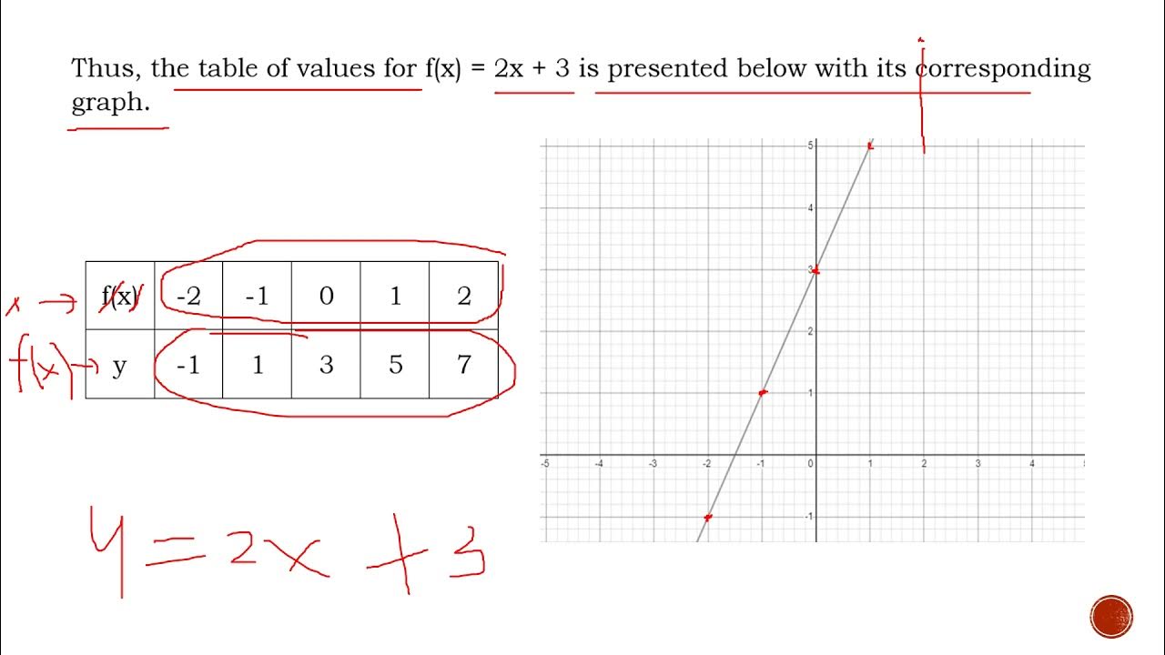
- 📊 To create a table for a rational function, substitute values of the independent variable into the function's equation and calculate the corresponding dependent variable values.
- 📉 The graph of a rational function will have vertical asymptotes where the denominator is zero, and these are represented by dashed lines on the graph.
- 🏃♂️ An example of a real-life application of a rational function is modeling the speed of a runner over time, with the function S(t) = 100 / t.
- 📝 When graphing, only positive values for time are considered since time cannot be negative.
- 📉 The graph of the runner's speed function will show how speed decreases as time increases.
- 🔄 Transformations of rational functions can involve horizontal shifts (changing the asymptote) and vertical shifts of the graph.
- 🔄 Changes in the denominator of a rational function can result in vertical shifts of the graph, while changes in the numerator can result in horizontal shifts.
- 📈 The graph of 1/x² is an example where the function does not have a negative denominator, and the graph is flipped on the x-axis compared to 1/x.
- 📚 The lesson concludes with a summary of how to represent rational functions and an invitation to check understanding through practice.
Q & A
What is the main objective of the lesson discussed in the transcript?
-The main objective of the lesson is to represent a rational function through its equation, table of values, and graph, and as a bonus, to discuss how to transform graphs of rational functions.
What is a rational function in mathematical terms?
-A rational function is a function of the form f(x) = P(x) / Q(x), where P(x) and Q(x) are polynomial functions and Q(x) is not equal to zero.
Why is it important to include negative, zero, and positive values when creating a table for a rational function?
-Including negative, zero, and positive values ensures that the behavior of the rational function is understood across the entire domain, except where the function is undefined (e.g., division by zero).
What is an asymptote and why is it significant in the graph of a rational function?
-An asymptote is a line that a graph approaches but never intersects. It is significant in the graph of a rational function because it indicates the values that the function approaches as the independent variable approaches infinity or negative infinity.
How does the value of a function become undefined in the context of rational functions?
-The value of a function becomes undefined when the denominator of the rational function is zero, as division by zero is undefined in mathematics.
What is the world record for the 100-meter dash as mentioned in the transcript, and who holds it?
-The world record for the 100-meter dash, as of October 2015, is 9.58 seconds, set by the Jamaican sprinter Usain Bolt.
How is the speed of a runner represented as a function of time in the transcript?
-The speed of a runner is represented as a function of time by the equation S(T) = 100 / T, where S is the speed and T is the time taken to run 100 meters.
What is the significance of the vertical dashed line in the graph of the function S(T)?
-The vertical dashed line in the graph of the function S(T) represents the time at which the speed would be undefined, which in this case is when T equals zero, as time cannot be negative.
What happens to the horizontal asymptote when a constant is added to the numerator of a rational function?
-When a constant is added to the numerator of a rational function, the graph of the function moves vertically by the same amount, and the horizontal asymptote also shifts by that constant value.
What is the effect of adding a constant to the denominator of a rational function on the graph and its vertical asymptote?
-Adding a constant to the denominator of a rational function shifts the graph horizontally. The vertical asymptote moves to the left by the absolute value of the constant if it's positive, or to the right if it's negative.
How does the exponent of the variable in the denominator affect the graph of a rational function?
-If the exponent of the variable in the denominator is even, the graph will not extend into the negative y-values, effectively flipping the lower half of the graph onto the x-axis.
What is the process of transforming the graph of the function f(x) = 1/x^2 when a constant is added to the function?
-When a constant is added to the function f(x) = 1/x^2, the graph moves vertically upward by the value of the constant. For example, if the function is g(x) = 1/x^2 + 2, the graph of g will be 2 units higher than that of f.
How does the graph of a rational function change when a constant is subtracted from the variable in the denominator?
-When a constant is subtracted from the variable in the denominator of a rational function, the graph moves horizontally to the right by the absolute value of the constant.
What is the final step in the process of representing a rational function through its equation, table of values, and graph?
-The final step is to connect the points plotted on the graph to visualize the behavior of the rational function, including its approach to any asymptotes.
Outlines

This section is available to paid users only. Please upgrade to access this part.
Upgrade NowMindmap

This section is available to paid users only. Please upgrade to access this part.
Upgrade NowKeywords

This section is available to paid users only. Please upgrade to access this part.
Upgrade NowHighlights

This section is available to paid users only. Please upgrade to access this part.
Upgrade NowTranscripts

This section is available to paid users only. Please upgrade to access this part.
Upgrade NowBrowse More Related Video
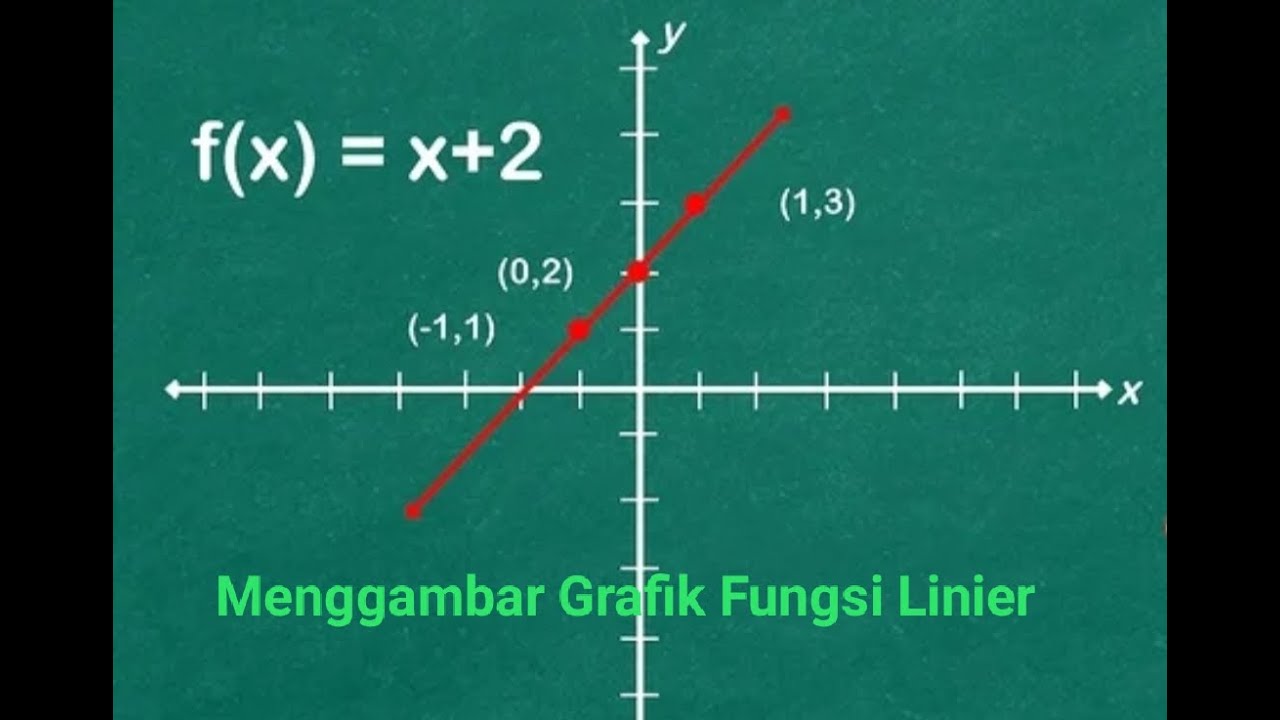
MaTek 1 Menggambar grafik Fungsi Linier #Part 6#Matematika Teknik 1
REPRESENT REAL-LIFE SITUATIONS USING RATIONAL FUNCTIONS || GRADE 11 GENERAL MATHEMATICS Q1
REPRESENTATIONS OF AN INVERSE FUNCTIONS | General Mathematics | Quarter 1 - Module 13
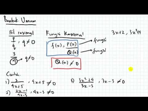
Fungsi Rasional kelas XI Matematika Tingkat Lanjut (Kurikulum Merdeka)
MCR3U (1.1) - Functions - relations, domain and range

SHS General Mathematics Q1 Ep2: Rational Functions
5.0 / 5 (0 votes)