#17 Solutions to LTI Systems | Linear System Theory

Summary

This lecture on Linear Systems Theory delves into state-space models and their solutions to differential equations. The instructor begins by reviewing foundational concepts from previous weeks, such as system properties and linear algebra tools. The core focus is on understanding the solution process for both time-invariant and time-varying systems, using Laplace transforms and matrix exponentials. A real-world example of an RL circuit illustrates the theory, explaining the evolution of current over time. The lecture emphasizes the natural and forced responses, setting the stage for deeper exploration of state-space models and control systems.

Takeaways

• 😀 Linear Systems Theory introduces state-space models to describe dynamic systems using differential equations.
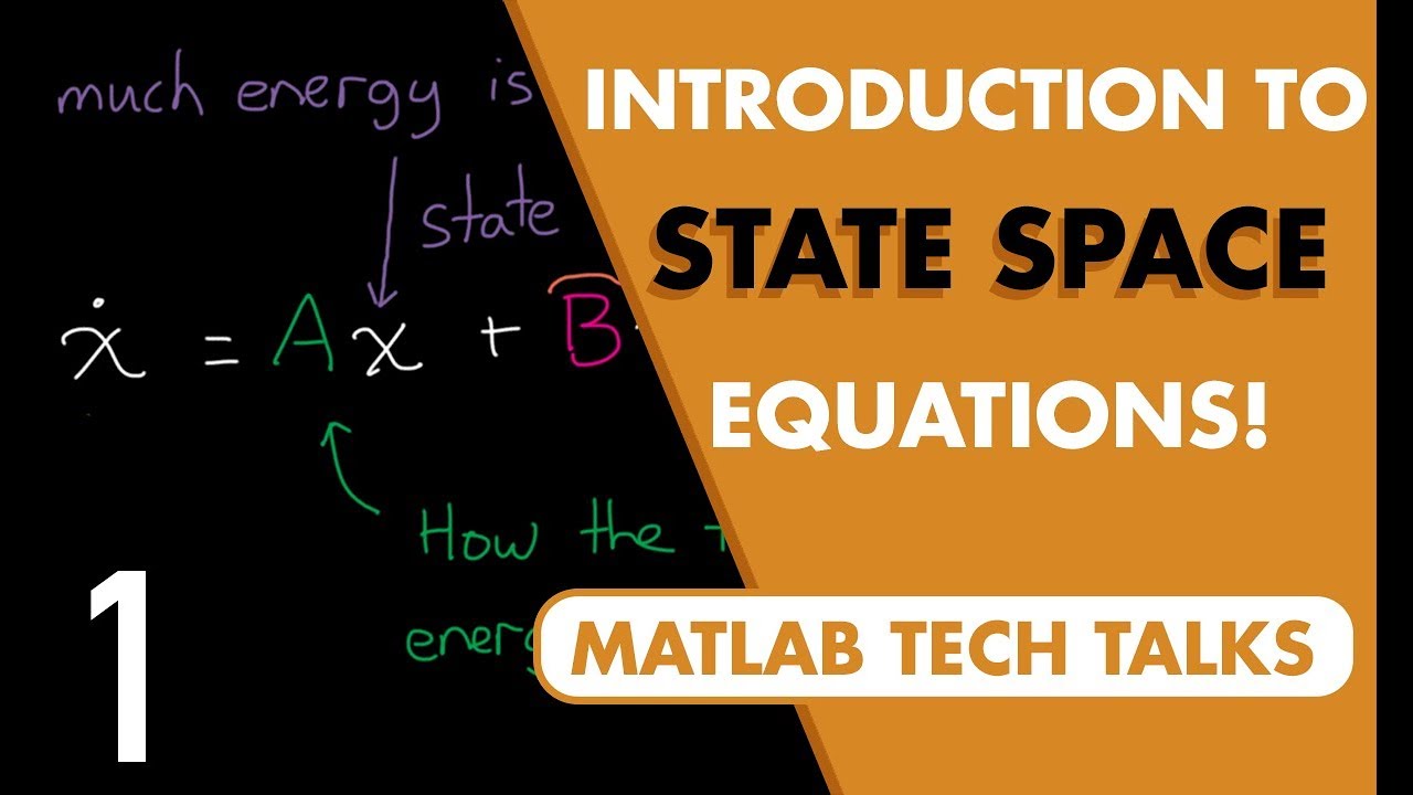
• 😀 State-space models are of the form ẋ = Ax + Bu, where A is the system matrix, B is the input matrix, and u is the control input.
• 😀 The lecture revisits the foundational tools of linear algebra, which are essential for solving state-space models in the course.
• 😀 The first part of the course focused on equipping students with necessary mathematical tools, which are now being applied to more complex systems.
• 😀 The lecture explains how to solve differential equations representing state-space models given initial conditions and control inputs.
• 😀 A real-world example using an R-L circuit helps illustrate the process of finding the evolution of current in the system over time.
• 😀 Solutions to these models can be decomposed into natural and forced responses. The natural response diminishes as time increases, while the forced response dominates in the steady-state.
• 😀 Laplace transforms are a valuable tool for solving differential equations, as they convert complex equations into simpler algebraic ones.
• 😀 In the case of a scalar system, the solution to the differential equation is represented by an exponential function e^(At), which evolves over time.
• 😀 For systems with multiple state variables (vector systems), the solution can be generalized using the matrix exponential e^(At), describing the system's evolution over time.
• 😀 The lecture sets the stage for solving more complex time-varying systems in upcoming sessions by first mastering the time-invariant cases.

Q & A

What is the focus of the course in Week 4?

Week 4 focuses on state space models and their solutions, particularly dealing with differential equations and understanding the state transition matrix. The lecture builds upon tools learned in linear algebra in previous weeks.

What are the two types of systems discussed in the lecture?

The two types of systems discussed are time-invariant and time-varying systems. The lecture starts with time-invariant systems and progresses towards time-varying systems.

How does the lecturer define a state space model?

A state space model is defined by the equation ẋ = Ax + Bu, where 'x' is the state vector, 'u' is the input, 'A' is the system matrix, and 'B' is the input matrix, which are of appropriate dimensions.

What is the key question the lecture attempts to answer regarding state space systems?

The key question is whether, given an initial state and a control input, it is possible to find the state of the system at any time 't' greater than 0.

What example is used to explain the application of state space models?

The example used is an R-L circuit with a constant voltage input. The goal is to determine the evolution of the current in the circuit over time, given the system parameters and initial conditions.

What mathematical technique does the lecturer mention for solving the differential equations?

The lecturer mentions using Laplace transforms to solve the differential equations. This method converts the differential equations into linear equations, making them easier to handle.

What are the two components of the system response discussed in the lecture?

The two components of the system response are the natural response (which accounts for the system's transient behavior) and the forced response (which is influenced by the external input, such as voltage in the case of the R-L circuit).

What does the natural response of the system depend on?

The natural response of the system depends on the system's initial conditions and decays over time in stable systems.

What is the significance of the term e^(-Rt/L) in the system's solution?

The term e^(-Rt/L) represents the decay of the natural response in the system. It appears in both the natural and forced components of the system's response, indicating how the system's behavior evolves over time.

How is the solution for a scalar system expressed in the lecture?

For a scalar system, the solution is expressed as a power series of time, where the coefficients can be determined by comparing both sides of the differential equation. The solution ultimately takes the form of e^(At), similar to the exponential function in standard scalar differential equations.