Microeconomics Unit 3 COMPLETE Summary - Production & Perfect Competition

Summary

In this microeconomics tutorial, Jer Breed explores production functions, marginal products, and costs for firms in perfectly competitive markets. The video covers the law of diminishing marginal returns, fixed and variable costs, and how they influence total costs. It explains the calculation of marginal cost, average costs, and how they intersect with marginal revenue for profit maximization. The tutorial also discusses long-term cost implications, economic vs. accounting profit, and how firms adjust to market changes to reach long-run equilibrium, emphasizing efficiency in perfectly competitive markets.

Takeaways

• 📊 The production function shows the relationship between the quantity of labor hired and the output produced, with diminishing marginal returns setting in as more workers are hired.
• 📈 Marginal product increases initially due to specialization, then decreases, and can eventually become negative as more workers are added.
• 💸 Fixed costs remain constant regardless of output, while variable costs increase as production increases; total costs are the sum of fixed and variable costs.
• 📉 Marginal cost is calculated as the change in total cost divided by the change in output and typically forms a U-shape on a graph.
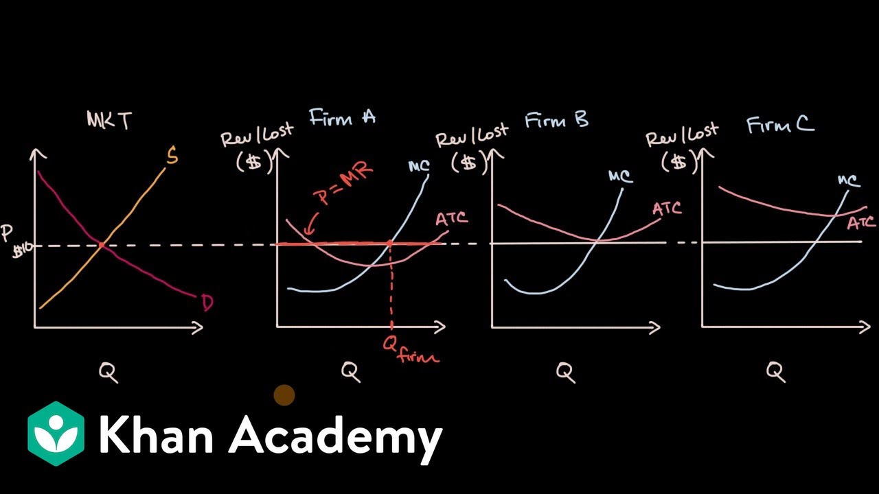
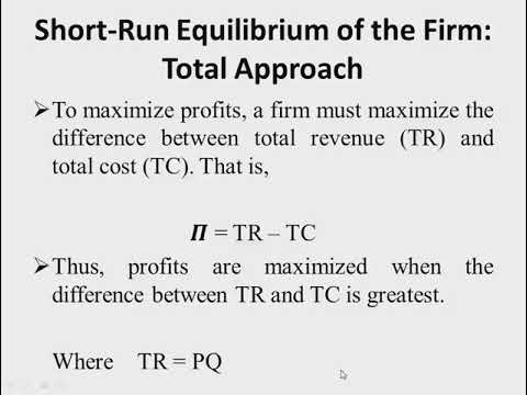
• ⚖️ Firms aim for profit maximization where marginal revenue equals marginal cost; this is the point at which producing more units is no longer profitable.
• 🏷️ In a perfectly competitive market, firms are price takers, selling identical products, with zero economic profit in the long run.
• 🔄 Long run costs involve all costs being variable, allowing businesses to change their production capacity by expanding factories or hiring more labor.
• 📉 Economies of scale allow firms to reduce average costs as they expand, while diseconomies of scale lead to higher costs as firms grow too large.
• 🧮 Economic profit considers both explicit and implicit costs, with zero economic profit known as normal profit.
• ⚙️ Perfectly competitive firms are both allocatively and productively efficient in the long run, producing at the lowest average total cost.

Q & A

What is the production function in microeconomics?

A production function shows the relationship between the quantity of labor a firm hires and the quantity of output produced by that labor. It illustrates how changes in labor affect total output.

What are the three phases of the law of diminishing marginal returns?

The three phases are: 1) Increasing returns: Marginal product rises as specialization occurs. 2) Diminishing returns: Marginal product falls but remains positive. 3) Negative returns: Marginal product becomes negative, decreasing total output.

How is marginal product calculated?

Marginal product is calculated by taking the change in total product and dividing it by the change in labor quantity. Since the change in labor is usually one worker, it equals the change in total product due to hiring an additional worker.

What is the difference between fixed costs and variable costs?

Fixed costs do not change with output, such as capital and land. Variable costs, like labor and electricity, change with the quantity of output produced.

What does the marginal cost curve represent, and how is it related to marginal product?

The marginal cost curve shows the cost of producing one additional unit of output. It is inversely related to marginal product; when marginal product rises, marginal cost falls, and when marginal product falls, marginal cost rises.

What is the relationship between marginal cost and average cost curves?

The marginal cost curve intersects the average variable cost and average total cost curves at their lowest points. When marginal cost is below the average cost, the average cost is falling. When it’s above, the average cost is rising.

What is the concept of productive efficiency?

Productive efficiency occurs when a firm produces at the lowest possible average cost. This happens at the minimum point of the average total cost curve, known as the productively efficient quantity.

How are economic profit and accounting profit different?

Accounting profit is calculated by subtracting explicit costs from total revenue. Economic profit also subtracts implicit costs (opportunity costs) from total revenue, making it a lower figure than accounting profit.

What is the profit-maximizing rule for firms?

Firms maximize profit by producing at the quantity where marginal revenue equals marginal cost. This ensures that the firm is not producing too much (increasing costs) or too little (missing out on revenue).

What are the characteristics of a perfectly competitive market?

In a perfectly competitive market, there are many firms selling identical products, with no influence on price (price takers), low barriers to entry, and zero economic profit in the long run due to competition.

Outlines

00:00

📊 Introduction to Microeconomics: Production and Competitive Markets

The video introduces the concept of production functions in microeconomics, focusing on the relationship between labor and output in perfectly competitive markets. It explains how a production function charts labor against output and calculates marginal product—the change in output from hiring additional workers. This section also covers the law of diminishing marginal returns, which states that after a certain point, adding more workers results in less efficient production, even leading to negative returns in some cases. A graph visualizing these concepts is introduced to better understand the dynamics of labor productivity.

05:03

💡 Fixed and Variable Costs Explained

This paragraph dives into the different types of costs in production: fixed costs (which do not change with output levels) and variable costs (which increase with higher output). Total cost is the sum of both fixed and variable costs. A graph is presented to illustrate the relationships between these costs and how they impact total production costs. Additionally, the marginal cost, which represents the cost of producing one more unit, is introduced alongside average variable cost and average total cost, explaining how they interact on a graph, especially at critical points such as when they intersect.

10:03

📉 Economies and Diseconomies of Scale

Here, the concept of long-run costs is explored, where all costs become variable as firms can change their capacity by expanding or contracting production. The paragraph introduces economies of scale, where increasing production lowers the average cost, followed by constant returns to scale, where production increases at the same rate as inputs. Finally, diseconomies of scale are discussed, where increasing production leads to inefficiencies, raising the average cost. These changes are explained through a graph that highlights long-run average total costs.

15:04

💰 Profit and Maximization in Business

This section focuses on profit maximization, comparing accounting profit (total revenue minus explicit costs) with economic profit (which also subtracts opportunity costs). It explains how firms aim to maximize profit by producing the quantity where marginal revenue equals marginal cost. The paragraph also covers normal profit, where economic profit is zero, and how businesses use marginal analysis to make production decisions. A graph illustrating profit-maximizing behavior in perfectly competitive firms is presented to show the relationship between costs, revenue, and output levels.

20:04

🏛️ Perfect Competition: Market Equilibrium and Efficiency

The final part explains perfect competition, where many firms sell identical products with no price control, leading to zero economic profit in the long run. It introduces the concepts of allocative and productive efficiency, explaining how in perfect competition, firms produce at both marginal cost and minimum average total cost in the long run. The paragraph also describes how supply and demand shifts bring firms back to long-run equilibrium, ensuring zero economic profit. Lastly, it discusses less common topics like increasing cost industries and the perfectly elastic long-run supply curve.

Keywords

💡Production Function

A production function is a model that shows the relationship between the quantity of labor a firm hires and the quantity of output that labor produces. In the video, the production function is represented by a chart that details how many units of output are produced with different quantities of labor. For example, with one unit of labor, 10 units of output are produced, illustrating the foundational concept of how production levels are determined by the amount of labor input.

💡Marginal Product

The marginal product refers to the additional output produced by using one more unit of input, or in this case, one more worker. The video explains how to calculate the marginal product by taking the change in total product and dividing it by the change in quantity of labor. It's a critical concept in understanding how production changes with additional labor and is used to illustrate the law of diminishing marginal returns.

💡Law of Diminishing Marginal Returns

This law states that as you add more of a single input (like labor) to a production process while holding other inputs constant, the additional output (or marginal product) will eventually decrease. The video describes this concept in three phases: increasing returns, diminishing returns, and negative returns, showing how the marginal product of labor changes as more workers are added.

💡Marginal Cost of Labor

The marginal cost of labor is calculated by dividing the wage paid to workers by their marginal product. It's depicted as an inverted version of the marginal product curve in the video. This concept helps to understand the cost implications of hiring additional workers and how it changes with different levels of production.

💡Fixed Costs

Fixed costs are expenses that do not change with the level of output. The video mentions capital and land as examples of fixed costs, which remain the same whether the firm produces nothing or a large quantity. These costs are crucial for understanding the total cost structure of a firm.

💡Variable Costs

Variable costs change with the level of output. As the video explains, these costs, such as labor and electricity, increase as more output is produced. Understanding variable costs is essential for calculating the total cost of production at different levels of output.

💡Total Costs

Total costs are the sum of fixed and variable costs. The video uses a table to illustrate how total costs are calculated by adding fixed costs to variable costs at different levels of output. This concept is vital for understanding the overall cost structure of production.

💡Marginal Cost

Marginal cost is the additional cost of producing one more unit of output. The video describes it as the change in total cost divided by the change in quantity. It's depicted graphically as a 'Nike Swoosh' shape, starting with a downward slope and then rising, which is crucial for understanding how costs change with increased production.

💡Average Variable Cost

Average variable cost is calculated by dividing the total variable cost by the quantity of output. The video explains that it decreases as more units are produced until it reaches a certain point, which is important for understanding how the cost per unit changes with scale.

💡Average Total Cost

Average total cost is the total cost divided by the quantity of output. The video describes how it changes with different levels of output and how it is represented graphically. This concept is key to understanding the average cost of production at various scales.

💡Productive Efficiency

Productive efficiency is achieved when a firm produces at the lowest possible average total cost. The video mentions that in the long run, perfectly competitive firms are productively efficient, producing at the minimum average total cost. This concept is important for understanding the optimal scale of production.

💡Perfect Competition

Perfect competition is a market structure characterized by many firms selling identical products, low barriers to entry, and no single firm influencing the market price. The video explains that in perfect competition, firms are price takers and earn zero economic profit in the long run. This concept is central to understanding how markets operate under ideal competitive conditions.

Highlights

Introduction to Unit 3 Microeconomics, focusing on production and perfectly competitive markets and firms.

Explanation of the production function: relationship between the quantity of labor hired and the output produced.

Definition and calculation of marginal product: change in total product divided by the change in labor quantity.

Description of the law of diminishing marginal returns, highlighting three phases: increasing returns, diminishing returns, and negative returns.

Marginal product curve explained, showing how it increases, then decreases, and eventually turns negative as more workers are hired.

Introduction to fixed costs (constant regardless of output) and variable costs (change with the quantity of output).

Total cost is the sum of fixed and variable costs; graphs show how fixed costs are horizontal, while variable costs increase with output.

Marginal cost is defined as the change in total cost divided by the change in quantity, showing a 'Nike Swoosh' shape in the graph.

Average variable cost and average total cost intersect marginal cost curves at their minimum points.

Key concept: productive efficiency occurs at the minimum average total cost, where the lowest production cost is achieved.

Discussion of economies of scale: larger businesses see lower average costs as output expands, explained through returns to scale.

Two types of profit: accounting profit (total revenue minus explicit costs) and economic profit (total revenue minus both explicit and implicit costs).

Firms maximize profits where marginal revenue equals marginal cost, a critical point in business decision-making.

Perfect competition described with key characteristics: many firms, identical products, low barriers to entry, and price-taking behavior.

Efficiency of perfectly competitive firms explained, with allocative efficiency and productive efficiency in the long run.

Transcripts

hi everybody Jer breed here from review

eon.com today we're going to be looking

at unit three for microeconomics this is

all about production and perfectly

competitive markets and firms this video

goes along with the total review booklet

from reviewe eon.com if you want to

purchase that head down to the links

below if you want to support this

Channel please like And subscribe as

well let's get into the content

first thing we're going to look at is

the production function a production

function shows the relationship between

the quantity of Labor a firm or business

hires and the quantity of output that

that number of workers produces here is

what it looks like on the chart we have

a table with the quantity of Labor this

is the number of workers hired and the

total product that's the number of units

of output these workers are able to

produce at one unit of Labor we will

have 10 units of output based on this

chart at two units of Labor we have 25

units of output at three units of Labor

we have 36 units of output four units of

Labor we have 46 units of output at five

units of Labor we've got 50 units of

output and at six units of Labor we drop

down to 48 in order to understand the

production function more clearly we need

to calculate the marginal product of

these workers to find the marginal

product you take the change in total

product and divide it by the change in

quantity since the change in quantity is

just one worker all the way through the

chart we're just looking at the change

in total product as a result of hiring

one more worker let's calculate it for

that first worker our total product goes

from zero up to 10 that's a marginal

product of 10 units of output for the

second worker our marginal product is 15

because we go from 10 total product up

to 25 total product keep on going and

our marginal product goes all the way

down to that last worker where we've got

-2 if we look at these numbers we see

three phases of the law of diminishing

marginal returns at the top those first

few workers that are hired we see

increasing Returns the total product is

increasing at an increasing rate

marginal product is rising we call that

increasing returns and it is as a result

of

specialization next we see the marginal

product starts to fall we call that

diminishing returns as we hire more

workers the marginal product Falls total

product is rising but at a decreasing

rate finally we see negative returns

that is where adding more workers

actually decreases total product

marginal product is negative let's take

a look at the graph here we have a

marginal product curve based on similar

numbers to what we just saw as you hire

more workers in the beginning the

marginal product increases then as you

hire more workers diminishing return

sets in and marginal product begins to

fall finally you have negative returns

as the marginal product is negative

those are the three phases of the law of

diminishing marginal returns in graph

form we can use the marginal product of

labor to calculate the marginal cost of

Labor in order to find that you take the

wage that you are paying your workers

and divide it by the marginal product of

those workers on the graph the marginal

cost of Labor looks like a flipped

upside down version of the marginal

product curve as the marginal cost of

Labor is downward sloping that is the

increasing returns phase of the marginal

product curve here we have

specialization causing the downward

slope of that marginal product of labor

curve as diminishing return sets in the

marginal cost of Labor curve upward

slopes that's diminishing returns now

we're going to look at two main

categories of cost for businesses first

we have fixed cost fixed costs are the

costs associated with production that

don't change with output producing zero

quantity of output is the same cost as

producing 100,000 quantity of output

Capital land those are both fixed costs

at least in the short run variable costs

on the other hand change with the co

quantity of output producing zero units

of output will have zero variable costs

producing five units of output will have

a much lower variable cost than

producing 100,000 units of output they

increase as more quantity of output is

produced things like labor electricity

those are variable costs and there are

lots of others total costs are fixed

costs and variable costs added together

two of those together give you your

total costs of production here we have a

table showing the values of fixed costs

variable cost and total costs for a firm

you'll notice the fixed costs don't

change the variable costs do change and

the total costs are always the fixed

cost and variable costs added together

if we graph it out it'll look something

like this the fixed cost is horizontal

because it doesn't change with the

quantity of output the variable cost

does change it starts off steep levels

off a bit and then tends to get steep

again generally speaking and you add

those two the variable cost and the

fixed cost together and that gives us

our total cost what that tells us is the

gap between the variable cost and the

total cost is the fixed cost here we see

in math form what marginal cost looks

like marginal cost is the change in

total cost divided by the change in

quantity here we're looking at the cost

of producing one more unit of output we

see our marginal cost of the first unit

is eight because our total cost goes

from $10 up to

$18 here we keep on going and we get the

overall marginal cost of production for

this firm if we graph it out it's going

to look like a Nike Swoosh it downward

slopes and then upward slopes next we're

going to calculate the average variable

cost how do you find the average of

anything divide by the quantity variable

cost of eight divided by a quantity of

one gives you a average variable cost of

eight keep on going down and you see

that all the way at six units the

average variable cost is $15 90 /

6 on the graph when we add the average

variable cost you'll notice that the

average variable cost intersects the

marginal cost curve at its minimum Point

make sure you notice that relationship

and remember it when you take your test

next we're going to look at the average

total cost just like before we're taking

the total cost and dividing by the

quantity because the average of anything

is the total of that thing divided by

the quantity here for

$18 with a quantity of one the average

total cost is 18 going all the way down

until we get to that sixth unit we're at

$16.70 worth of average total cost if we

add it to the graph we'll notice that

there's a similar relationship between

the average total cost and that marginal

cost as the marginal cost curve is below

the average total cost the average total

cost is falling once that marginal cost

is above the average total cost the

average total cost is rising that

relationship is important and make sure

you remember it on your next test and

that means that the average total cost

intersects the marginal cost curve at

its minimum point one thing to note is

the quantity at the minimum point of the

average total cost curve is called

productively efficient that is the

quantity that has the lowest average

cost of production productively

efficient so how do you find the average

fixed cost for this firm well the

average fixed cost is the gap between

the average total cost and the average

variable cost so that Gap right there is

your average fix cost you can find it at

any quantity so how would you be able to

find the total cost when you have a

graph like this showing average cost and

marginal cost well the total cost of

anything is the average of that thing

times the quantity so pick a quantity

and there we can go on up at this q1

point we have our average variable cost

there at P1 that gives us this square

right here of variable cost we could

calculate the area of that if there were

numbers and that would give us our total

variable cost if we keep on going up to

P2 at the average total cost there

calculate the area of that rectangle and

we will have our total cost how do we

find the fixed cost well it's the gap

between the two that rectangle there is

our fixed cost for q1 now those cost

curves can shift if there's a change in

production cost if there's a change in

fixed cost like advertising new

production equipment being purchased

that would move the average total cost

curve only only up with an increase down

with a decrease if we have a change in

variable cost that'll move the average

total cost curve the average variable

cost curve and the marginal cost curve

now let's look at long run costs in the

long run all costs are variable variable

costs are variable but fixed costs are

also variable because in the long run I

can buy new plants and equipment I can

also open up new stores new factories or

whatever it may be in the short run we

can change the rate of production I can

hire more workers I can speed up my

production I can slow down my production

I can produce more or less in the short

run long run changes are about capacity

of production if I'm opening up new

businesses opening up new plants or

factories that is a change in the

maximum production level of my business

and that is a capacity long run change

here's what long run costs look like on

the graph we get a long run average

total cost curve as a business EXP

expands into a larger and larger

business opening up new factories and

plants we see a downward sloping portion

of the long run average total cost curve

here average costs are falling we call

that economies of scale mathematically

we could call it returns to scale

doubling all of the inputs land labor

and capital will get more than double in

new output and we call that increasing

returns of scale average costs are

falling as this firm continues to expand

it's going to have a horizontal portion

of its long run total cost curve and

there we have constant returns to scale

as this firm continues to produce more

and more output it is doubling its

inputs and getting exactly double output

we call that constant returns to scale

average costs are staying constant most

businesses will eventually reach a point

where average costs in the long run

begin to rise the business is now

growing too large and it's becoming an

inefficient bureaucracy

here we call this diseconomies of scale

long run average costs are beginning to

increase as production is expanded we

call that decreasing returns to scale

mathematically you double your inputs

and get less than double for output next

we're going to look at profit remember

profit maximization is a basic

assumption in AP economics firms seek a

profit there are two types of profit the

first one is called accounting profit

the second one is called economic profit

now obviously since this is economics

that e economic profit is probably more

important but accounting profit shows up

on exams and you need to know it here's

the formula for accounting profit you

take the total revenue price times

quantity then you subtract your explicit

costs that's money paid by the

entrepreneur to operate their business

it's money directly out of their pocket

now economic profit is a lower number

and the reason why is because economists

will subtract not just the explicit cost

from total revenue but also the implied

costs entrepreneurs have opportunity

costs and we need to subtract those

opportunity costs to find the true

economic profit just so you're aware

there are explicit and implicit variable

costs and fixed costs so in those cost

curves we already looked at before there

are explicit and implicit costs within

all of those you may see a term normal

profit on your next exam normal profit

means that economic profit is zero it

means that accounting profit is equal to

the implicit costs of production next

we're going to look at production

decisions for individual businesses or

firms this is an application of marginal

analysis that you already learned about

back in unit one remember marginal

benefit equals marginal cost that is

your benefit maximizing Behavior but for

businesses we don't really look at

marginal benefit in business a firm's

benefit is revenue marginal revenue is

the change in total revenue divided by

the change in quantity this is the

Revenue brought in for producing one

more unit of output The Profit

maximizing quantity for a firm is found

and make sure that you write this down

because it's important it is found where

marginal revenue equals

margin where marginal revenue equals

marginal cost make sure you remember

that it shows up on the exam over and

over and over here's what it looks like

on the graph we have our marginal

revenue curve for a perfectly

competitive firm and we have our

marginal cost curve at lower quantities

here the marginal cost is less than the

marginal revenue that means this firm

will increase profit by continuing to

produce more units of output at higher

units of output we see that the marginal

cost is now greater than the marginal

revenue there the firm is losing profit

by increasing production they should

produce less The Profit maximizing point

is where marginal revenue equals

marginal cost it's where those two

curves intersect make sure you remember

that and jot it down because it'll be on

your test for sure now we're on to our

last topic this is perfect competition

you've already learned a little bit

about perfect competition it's the

supply and demand graph that you learned

back in unit 2 here are the qualities of

a perfectly competitive market we have

lots and lots of firms within this

Market they're also selling identical

products that means there's no name

brands or advertisements to distinguish

between the different products that are

available we also have low barriers to

entry that low barriers to entry means

that firm firms enter when others are

making profit and firms exit when others

are suffering economic losses that means

there is zero economic profit in the

long run for perfectly competitive firms

the last thing is that these firms have

no influence on price they are price

takers that means the market equilibrium

Price sets the price that each firm can

charge within a perfectly competitive

market you've already seen the market

graph for perfect competition we have a

downward sloping demand curve upward

sloping supply curve and that

intersection between those two curves

gives us our equilibrium price that

equilibrium price goes on over to the

firm graph and gives us our marginal

revenue curve it's the demand for the

firm that firm can sell as many units of

output as it wishes at that market price

that gives us our demand average revenue

and price we call it Mr darp now let's

throw on the other cost curves we

learned earlier at the intersection

between the marginal cost and the

marginal revenue curve we get a profit

maximizing quantity labeled qf here

since this firm's average total cost

curve is below the marginal revenue

curve at that profit maximizing quantity

this firm is earning an economic profit

you can always tell that a firm is

making an economic profit if the average

total cost is less than the equilibrium

price from the market at the firm's

profit maximizing quantity here we have

another firm and this firm is earning

economic losses the reason we know that

is because the average total cost curve

is greater than the equilibrium price

from the market now we have another

graph here this firm is earning zero

economic profit it's breaking even it's

earning a normal profit all of those are

the same thing and we call this long run

equilibrium because firms will earn zero

economic profit in a perfectly

competitive market in the long run so in

the long run the price from the market

equals the minimum of the average cost

curve make sure you know how to draw all

three of these graphs profit loss and

breaking even which is long run

equilibrium

next we're going to look at how firms

get to that long run equilibrium if they

are earning economic profits to start

this firm here is earning an economic

profit that economic profit is going to

cause firms to seek that profit firms

enter the market as a result in the

market that causes the supply curve to

shift to the right driving the price

down and increase in the quantity in the

market for the firm that causes the

marginal revenue demand average revenue

and price Mr darp to fall downward until

it reaches the minimum of the average

total cost curve special note when

you're drawing these graphs it goes

further than the bottom of that profit

box next we're going to look at a firm

that is earning economic losses those

economic losses will cause firms to exit

the market in the long run as firms exit

the market that causes the supply curve

to shift to the left driving the price

up and decreasing the equilibrium

quantity within the market back on the

firm graph the increase in the

equilibrium price from the market shifts

the Mr Dar marginal revenue demand

average revenue and price upward until

it hits the minimum of the average total

cost curve and there we are back at long

run equilibrium the firm is earning a

normal profit once again next we're

going to talk about efficiency for

perfectly competitive firms there are

two types of efficiency don't forget

there's allocative efficiency and

there's productive efficiency perfectly

competitive firms are allocatively

efficient in the long run and the short

run because price always equals marginal

cost for productive efficiency perfectly

competitive firms are productively

efficient in the long run because they

produce at the minimum average total

cost in the long run in the short run

that isn't true when the firm is earning

either economic losses or economic

profits the firm's average total cost is

greater than the minimum average total

cost we're going to take a step back for

just a moment and look at a firm's short

run supply curve here we have a graph

for a firm and we have the profit

maximizing quantity of qf at the current

equilibrium price the firm is currently

in Long Run equilibrium we're going to

add a point here because this is the

quantity that this firm would produce at

the current equilibrium price that is

one of the points on this firm's supply

curve if the price goes up the firm will

be earning economic profits in the short

RM run and they will produce a higher

quantity at that higher price that's our

second point on the firm's short run

supply curve if there was a decrease in

the equilibrium price from the market

The Firm would now be producing a lower

quantity qf there at the new lower price

this firm is now earning economic losses

but they aren't going to shut down

because these economic losses are less

than they would be if they shut down

because if the firm shuts down it has to

pay its fixed costs and the fixed costs

are larger than the current economic

losses that means that if the price is

above the average variable cost this

firm loses less than its fixed cost so

the firm should go ahead and operate if

the price Falls a little bit further now

we are at the minimum of the average

variable cost this is the lowest price

this firm would willingly produce that

is the last point on our supply curve

for this firm this firm's supply curve

is the marginal cost curve above the

minimum of the average variable cost

before we finish up we're going to go

over two less common topics the first

one of those is increasing cost

Industries if you ever see any questions

about that and they're rare just know

that if there's an increase in the

number of firms within the market each

individual firms cost curves shift up

that's an increasing cost industry the

next thing we're going to look at is the

long run supply curve in a perfectly

competitive market it's not the upward

sloping supply curve we have there and

here's why because here is our current

equilibrium output and price we're going

to go ahead and put a point there that

is one of the points on our long run

supply curve because this firm is

currently in Long Run equilibrium let's

say there's an increase in demand

in this market when the demand increases

that causes an increase in the

equilibrium price causing the firm to

earn economic profits in the short run

in the long run firms are going to enter

the market driving the price back down

to where it was previously we now have a

higher quantity at the exact same price

that is our second point on our long run

supply curve let's go back to where we

started for a moment and this time we

are going to show a decrease in demand

that causes the price in the market to

fall on the firm graph that causes the

firm to earn an economic loss in the

short run those economic losses Drive

firms out of the market that causes the

supply curve to shift back to the left

bringing the price back to where it was

previously where we have a new lower

quantity at the same price that gives us

a third point on this long run supply

curve for this Market connect all of

those points together and that gives us

a horizontal long run supply curve it is

at the minimum of the average total cost

curve for the firm that's where you find

the markets long run supply curve it's

perfectly elastic because in the long

run a perfectly competitive market will

produce any output at that

price we got through it that was a lot

of information there and if you knew it

all you are on your way to acing your

next exam if you need a little more help

head down to the links below where there

are lots of games and activities from

reviewe eon.com to help you study and

practice the skills you need for that

next exam if you want to support this

channel make sure you like And subscribe

and then head over to reviewe eon.com

and pick up the total review booklet

with everything you need to know to pass

your final exam or AP economics exam

thank you very much I'll see you guys

next time