But what is a convolution?
Summary
TLDRこのビデオスクリプトでは、異なる数値リストや関数を組み合わせる方法の一つとして、あまり一般的でないが基本的な「畳み込み」に焦点を当てています。畳み込みは画像処理、確率論、微分方程式の解法など、多岐にわたる分野で重要な役割を果たしています。具体的には、2つのサイコロの確率分布を畳み込む例や、ポリノミアルの乗算、移動平均、画像のぼかし効果などの計算方法を通じて、畳み込みの直感的な理解を深めることを目指しています。さらに、高速フーリエ変換を利用した畳み込みの効率的な計算方法についても触れ、数学が多様な分野でどのように応用されるかを示しています。
Takeaways
- 😀 Convolution is a fundamental way to combine two lists or functions
- 😀 Useful in many areas like image processing, probability, differential equations
- 😀 Can visualize as sliding windows or table of products
- 😀 Blurring images is like a weighted moving average
- 😀 Choosing different kernels gives different effects
- 😀 Connected to multiplying polynomials and collecting terms
- 😀 Using FFTs gives a faster convolution algorithm
- 😀 Leverages structure of roots of unity evaluation points
- 😀 Speedup helps many applications needing convolution
- 😀 Even relates to standard multiplication of numbers
Q & A
畳み込みとは何ですか?
-畳み込みは、二つのリストや関数を組み合わせて新しいリストや関数を生成する方法の一つであり、各項を個別に加算や乗算する以外の方法で、一方の配列を反転させて他方との各項の積を取り、それらを加算して新しいシーケンスを作成します。
畳み込みの応用分野はどこにありますか?
-畳み込みは画像処理、確率論、微分方程式の解法など、多岐にわたる分野で広く使用されています。特に、多項式の乗算において畳み込みが自然に現れます。
畳み込みが確率論でどのように使用されるかの具体例は?
-畳み込みは、異なる確率分布の合成を計算する際に使用されます。例えば、二つのサイコロを振ったときの目の和の確率分布を求めることができます。
畳み込みを計算するためのアルゴリズムは?
-畳み込みを計算するためのアルゴリズムには、直接的な方法と、FFT(高速フーリエ変換)を利用した方法があります。FFTを用いた方法は計算効率が良く、特に大きなデータセットに対して高速に畳み込みを計算できます。
畳み込みの直感的な理解はどのように得られますか?
-畳み込みの直感的な理解は、一方の配列を反転させ、それを他方の配列に沿ってスライドさせながら、重なる部分の要素同士を乗算し、その積を加算することで新しい配列を生成するプロセスを可視化することで得られます。
画像処理における畳み込みの役割は?
-画像処理において、畳み込みは画像の平滑化(ブラーリング)、エッジ検出、シャープ化などの効果を実現するために使用されます。これは、特定のカーネル(小さな行列)を画像全体に適用することで行われます。
畳み込みニューラルネットワークとは何ですか?
-畳み込みニューラルネットワーク(CNN)は、畳み込みの概念を利用した深層学習のモデルの一つで、特に画像認識や音声認識などの分野で優れた性能を発揮します。CNNは、データから自動的に特徴を抽出する能力を持っています。
多項式の乗算に畳み込みがどのように関連しているか?
-多項式の乗算は、その係数の畳み込みによって計算できます。これは、多項式の各項を乗算し、同じ次数の項を加算するプロセスが、畳み込みの定義と一致するためです。
畳み込みの出力の長さはどのように決まりますか?
-畳み込みの出力の長さは、入力された二つの配列の長さに依存します。一般的に、出力の長さは入力配列の長さの合計から1を引いたものになります。ただし、実際の応用では出力を特定の長さに調整するために切り捨てやパディングが行われることがあります。
畳み込みを利用したアルゴリズムの計算効率について説明してください。
-畳み込みを直接計算する方法は一般にO(n^2)の計算量がかかりますが、FFTを利用した畳み込み計算はO(n log n)の計算量で済み、大規模なデータに対してはこの方法が非常に効率的です。
Outlines

このセクションは有料ユーザー限定です。 アクセスするには、アップグレードをお願いします。
今すぐアップグレードMindmap

このセクションは有料ユーザー限定です。 アクセスするには、アップグレードをお願いします。
今すぐアップグレードKeywords

このセクションは有料ユーザー限定です。 アクセスするには、アップグレードをお願いします。
今すぐアップグレードHighlights

このセクションは有料ユーザー限定です。 アクセスするには、アップグレードをお願いします。
今すぐアップグレードTranscripts

このセクションは有料ユーザー限定です。 アクセスするには、アップグレードをお願いします。
今すぐアップグレード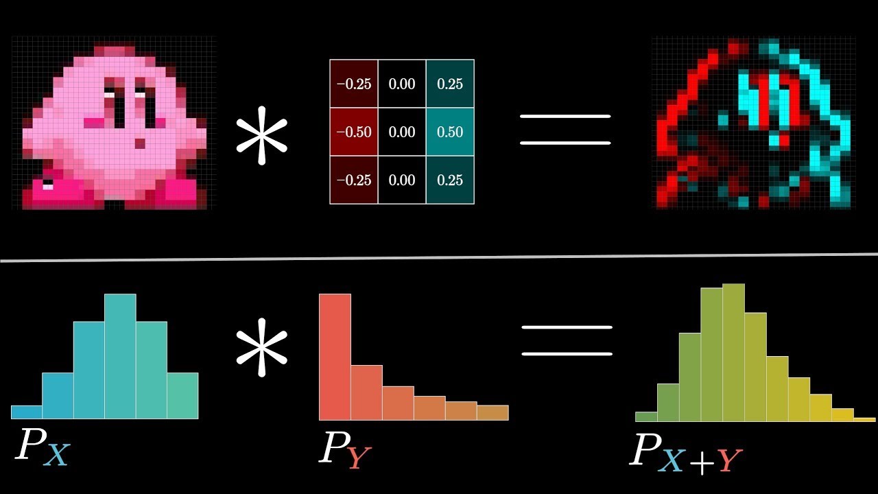


5.0 / 5 (0 votes)