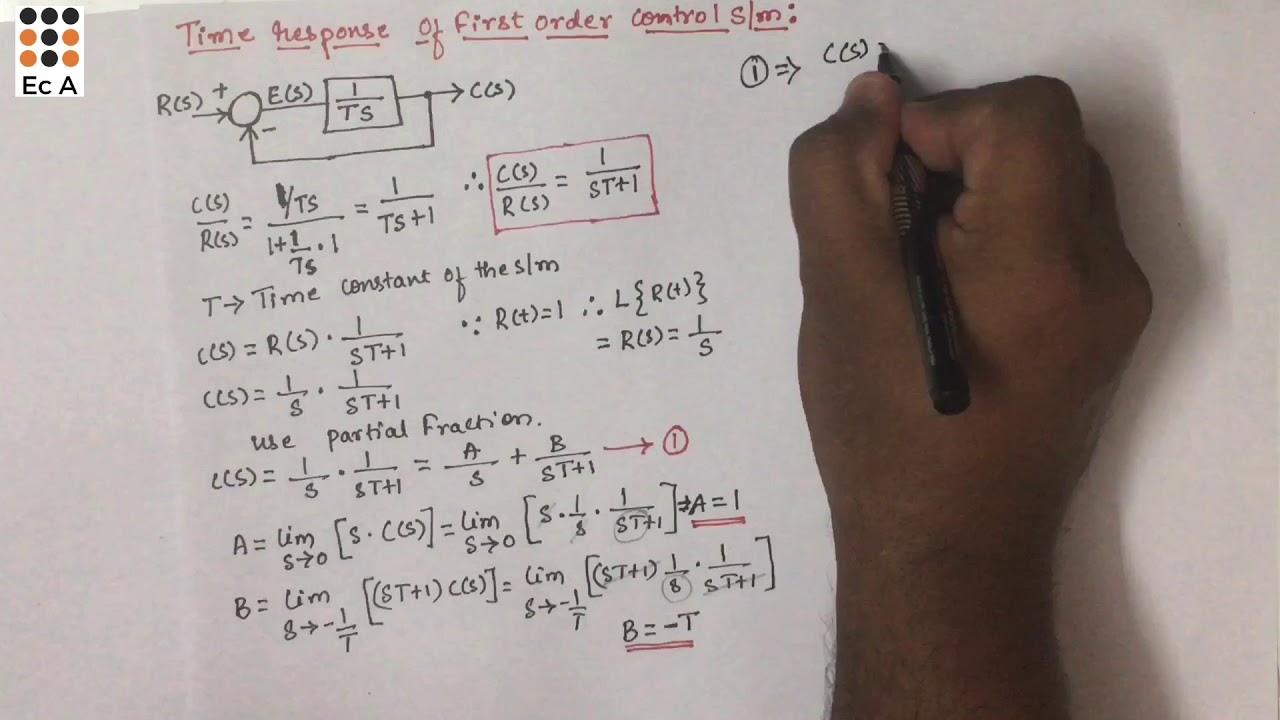
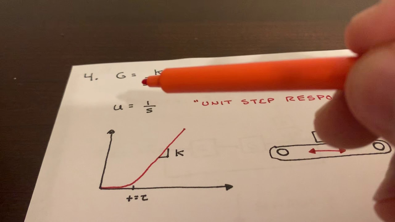
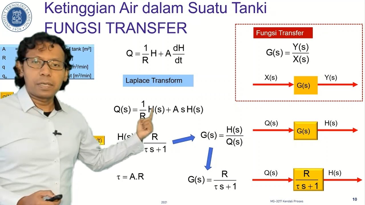
ECE 461.11 First and Second Order Approximations

Summary

In ECE 461 Lecture 11, the focus is on first and second order approximations for control systems. The lecture explains the concept of dominant poles, which are crucial for simplifying high-order systems while preserving their behavior. It covers how to identify these poles and match the DC gain for an accurate model. The importance of settling time, overshoot, and damping ratio is discussed, with methods to determine these parameters from a system's step response. The lecture also touches on the practical use of these concepts in real-world applications, such as car suspensions and missile systems.

Takeaways

• 📚 The lecture introduces first and second order approximations for control systems, emphasizing the impracticality of manually calculating higher order systems like the 250th order Maverick missile model.
• 🔍 The concept of dominant poles is highlighted as crucial in understanding system responses, where one or two poles usually have the most significant impact on the system's behavior.
• 🚗 An example is given using a car's vibrational modes to illustrate how the lump mass of the car represents the dominant pole in its response to road conditions.
• 🔑 The importance of modeling is underscored, with the goal of creating a simpler yet accurate representation of a system by matching the dominant pole and DC gain.
• 📉 Definitions of key terms such as 'dominant pole', 'DC gain', 'two percent settling time', 'overshoot', and 'damping ratio' are provided to establish a foundation for understanding control systems.
• 📈 The process of identifying the dominant pole is explained, often being the pole closest to the origin, and its significance in creating a simplified model of the system.
• 📝 The method of determining system parameters from the step response is demonstrated, showing how the DC gain and settling time can be used to infer the system's characteristics.
• 🔄 The script discusses how to handle complex poles, which require considering both the real and imaginary parts to understand the system's behavior fully.
• 📊 The relationship between the damping ratio and overshoot is detailed, explaining how the damping ratio can be used to predict the system's stability and response to changes.
• 📚 A summary of second order systems is mentioned, which would likely include graphical representations and tables for quick reference in determining system characteristics from response data.
• 🔧 The lecture concludes with an overview of how to use the information about dominant poles and system responses to approximate and understand the behavior of more complex systems.

Q & A

What is the main purpose of identifying dominant poles in control systems?

The main purpose of identifying dominant poles is to simplify the analysis of a system by focusing on the poles that significantly influence the system's response, allowing for a more manageable and accurate model.

Why is it impractical to find the step response for very high order systems by hand?

Finding the step response for very high order systems by hand is impractical because it becomes extremely complex and time-consuming, and it can lead to a loss of intuitive understanding of the system's behavior.

What is meant by the term 'DC gain' in the context of control systems?

The DC gain refers to the gain of a system at low frequencies, specifically at s equals zero, which indicates the system's steady-state response to a constant input.

How is the two percent settling time defined in control systems?

The two percent settling time is defined as the time it takes for the system's response to reach and stay within 2% of the final steady-state value, which is a standard used for simplicity in calculations.

What is the significance of the damping ratio in control systems?

The damping ratio is significant as it indicates the amount of overshoot in the system's response to a step input, which is crucial for designing systems with desired stability and performance characteristics.

How can the dominant pole be determined for a system with multiple poles?

The dominant pole can be determined by analyzing the system's step response or by identifying the pole closest to the origin, as it usually has the largest initial condition and decays the slowest, thus having the most significant impact on the system's response.

What is the relationship between the dominant pole and the system's step response?

The dominant pole largely dictates the behavior of the system's step response, including the speed of response and the amount of overshoot, making it a key factor in system modeling and analysis.

Why might a simplified model that retains the dominant pole and matches the DC gain be considered 'good enough' for many applications?

A simplified model that retains the dominant pole and matches the DC gain is considered 'good enough' because it captures the essential behavior of the system, providing an 80-85% accurate representation that is both manageable and useful for most practical purposes.

How can complex poles be handled in the context of system modeling and approximation?

Complex poles can be handled by ensuring that their complex conjugate is also included in the model, effectively treating them as a second-order system for the purpose of approximation and analysis.

What is the concept of time scaling in control systems, and why is it used?

Time scaling is the concept of adjusting the time units used in system analysis to align the dominant pole with a more manageable location, typically near minus one, simplifying calculations and making the system's behavior more intuitive.

How can the step response of a system be inferred from its transfer function without explicitly calculating it?

The step response can be inferred by examining the transfer function's dominant pole and DC gain, as these parameters provide insights into the system's settling time and steady-state behavior, allowing for an estimation of the step response characteristics.

Outlines

00:00

🔍 Simplifying High-Order Systems

The lecture discusses the challenge of finding the step and impulse responses for high-order systems, such as a 250th order system. It introduces the concept of dominant poles, which are the poles that significantly influence a system's response. By focusing on these dominant poles and the DC gain, a simpler yet accurate model can be developed. This method retains the essential behavior of the system while making analysis more manageable.

05:00

🖥️ Comparing First and Higher-Order Models

This section compares the step responses of higher-order systems with simplified models that retain the dominant pole and DC gain. The lecture demonstrates that the responses of a complex system and its first-order approximation are nearly identical, except for slight delays. It emphasizes the utility of modeling complex systems with simplified approximations for practical analysis, especially when dealing with systems that include complex poles.

10:01

⚙️ Understanding Dominant Poles in System Approximation

Here, the focus is on how dominant poles can be identified and used to approximate a system's behavior. The lecture explains the process of determining the dominant pole by analyzing the step response and how this information can be used to create simplified models. It covers both real and complex poles, detailing how the DC gain, settling time, and frequency of oscillation are crucial parameters in this analysis.

15:04

📊 Second-Order Systems and Damping Ratio

The lecture concludes with a detailed explanation of second-order systems, focusing on the damping ratio and its impact on system behavior, including overshoot and resonance. It explains how to derive system parameters from the step response and how to use damping ratio values to predict system behavior. The section also introduces Bode plots and their relevance in control systems, setting the stage for future lectures.

Keywords

💡Control Systems

Control systems are the central theme of the video, referring to the set of components that manage and command the behavior of other devices or systems. In the context of the video, control systems are used to analyze and design the behavior of dynamic systems, such as the response to a step input, which is a common way to test system performance.

💡Step Response

The step response is a fundamental concept in control systems, representing the reaction of a system to a sudden change in input, or a 'step' function. The video discusses how to find the step response for a transfer function and the challenges of doing so for high-order systems, emphasizing the importance of understanding the step response for system analysis.

💡Impulse Response

Impulse response is another key concept in control systems, which is the system's reaction to a brief input signal or 'impulse'. While the video mentions it in the context of finding responses for transfer functions, the focus is on step response due to its practical significance in system behavior analysis.

💡Dominant Pole

A dominant pole is a pole in the system's transfer function that has the most significant effect on the system's response. The video explains that for most systems, there are one or two poles that dominate the response, and understanding these can simplify the modeling and analysis of complex systems.

💡DC Gain

DC gain is the gain of a system at very low frequencies, specifically when s equals zero in the Laplace domain. The video mentions matching the DC gain as a crucial step in creating simplified models that maintain the essential characteristics of the original system.

💡Settling Time

Settling time is the duration it takes for a system's response to reach and stay within a specified percentage of its final value after a step input. The video uses the two percent settling time as a standard, which is a common engineering practice to define when a system has sufficiently settled.

💡Overshoot

Overshoot is the amount by which a system's response exceeds its final steady-state value before settling. The video discusses overshoot in the context of system performance, such as in an egg polisher where no overshoot is desired to prevent damage.

💡Damping Ratio

The damping ratio is a measure of how oscillations in a system decay over time. It is defined as the cosine of the angle of the pole in the complex plane. The video explains how the damping ratio relates to overshoot and is essential for designing systems with desired dynamic behavior.

💡First and Second Order Approximations

First and second order approximations are simplified models of systems that capture the dominant dynamics. The video focuses on these approximations as a means to understand and model systems with complex dynamics by focusing on the dominant pole and matching the DC gain.

💡Transfer Function

A transfer function is a mathematical representation that relates the input and output of a system in the frequency domain. The video discusses how the transfer function is used to analyze the behavior of control systems and how it can be simplified by focusing on the dominant pole.

💡Time Scaling

Time scaling is the concept of adjusting the time units used to analyze a system, which can affect the apparent position of the dominant pole. The video mentions that systems in the class typically have dominant poles near minus one, which can be a result of time scaling to make mathematical analysis easier.

Highlights

Introduction to Lecture 11 on first and second order approximations in control systems.

Explanation of why manually finding the step response for high order systems is impractical and the importance of dominant poles.

Dominant poles are the key factors that dictate the system's response, often being the poles closest to the origin.

The concept of modeling to simplify complex systems while retaining accuracy and manageability.

Matching the dominant pole and DC gain for an accurate system model.

Definition of DC gain as the gain at s equals zero.

Discussion on the two percent settling time and its significance in system response.

The impact of overshoot in system design, with examples like egg polishers and car suspensions.

How to determine the dominant pole in a system with multiple poles.

Simplification of a system by keeping the dominant pole and adjusting the DC gain.

Demonstration of how a simplified model can closely resemble a complex system's step response.

Approach to handling complex poles and their conjugates in system modeling.

The process of finding the transfer function from a given step response.

Explanation of how to calculate the settling time and frequency of oscillation from a pole's properties.

Introduction to damping ratio and its role in determining overshoot.

The use of time scaling to normalize dominant pole positions for easier calculations.

Different ways to represent second order systems and how to determine them from system responses.

Summary of the lecture providing insights into the practical applications and theoretical foundations of first and second order system approximations.

Transcripts

welcome to ece 461

control systems lecture number 11 first

and second order approximations

now in the previous lecture we looked at

how to find the step response

and impulse response for a transfer

function

that gets really unwieldy when you start

getting your eighth ninth tenth order

systems

that actually can happen the maverick

missile for example

was modeled as a 250th order system i

don't really want to find the step

response of a 250th order system by hand

plus you lose all intuition if i look at

this transfer function and said

by inspection what's the step response i

really have no idea

so there's the trick when you have a

dynamic system

there's a few poles that really dominate

the response

those the dominant poles what i'd like

to do is take this system

and come up with model which is simpler

but still fairly accurate and he has a

similar step response

keeping the same dominant pole does that

so the concept of what a dominant pole

is for most systems

there's one or two poles that tend to

really dominate the responsive system

for example with my car as you're going

down the road there's vibrational modes

twisting modes

a lot of rattling all those are pulls

the lump mass of the car really

dominates the response however

so if i just modeled that one pole the

lump mass

i'd have a pretty good model for the

system and that's really the purpose of

modeling

how do i come up with a mathematical

model which is simple

meaning useful but still fairly accurate

the idea is if i match the dominant pole

and match the dc gain

i've got a model that's you know really

pretty good you know 80 85 percent

correct

plus it's manageable if when you get a

more accurate model

best read through it throw it into a

computer simulation or matlab

so a couple definitions to start out the

domino pole

is the pole that dominates response

which is kind of a tautology

it's if you look at the step response

there's the overall

response that's uh really dictates how

it behaves

that's the dominant pole usually is the

pole closest to the origin

not always but usually the transfer

function

is the differential equation that

relates the input in the output

the dc gain is the gain at dc at s

equals zero

the two percent settling time is the

differential equation

it'll respond and in theory takes

infinite time to settle out

infinity is not a terribly easy number

to use so what i do

is come up with a way of saying as soon

as i get close to zero

i'll call that the settling time and to

define close

that's kind of arbitrary typically two

percent settling time is used

the reason being is two percent's got a

nice logarithm the log of 0.02 is minus

4.

so back in the days of slide rules

logarithms were painful to use

so they use something that has got a

nice logarithm and that standard is

stuck

overshoot if i have a step response is

how much it overshoots

sometimes that's really important for

example if i want to have an egg

polisher

i want to have no overshoot because i'll

crack the egg if your car hits a pothole

you want it to bounce about three times

for about 30 of your shoot

typically when you specify how the

system should behave you specify the

overshoot and the settling time

from that i've got to translate it to

control systems terms

the damping ratio is the angle of the

pole cosine of the angle is your zeta

the damping ratio damping ratio tells

you the overshoot

uh so if i have a system i've got to

figure out which one is the dominant

pole

as i mentioned it's the one closest to

the origin and you can see that here

suppose i have three poles one minus one

minus ten minus one hundred

which one's dominant well one way to do

that is take the step response

i'll apply a step input do your partial

fraction expansion

and it says here's your step response

the 2 is the forced response

that comes from my step input these are

the transients

and if you notice this term in the

transient that first one

it really dominates it starts out 10

times larger than

anyone else plus it lasts 10 times

longer

so this is called the dominant pole

almost invariably it's the pole closest

s equals zero

the reason being is this input this

forcing function excites these poles

the pull closest to it has the largest

excitement

largest initial condition and it decays

the slowest

kind of gives you a double whammy the

largest initial condition flash the

longest

is the dominant pole

with that i can do things and come up

with a simplified model

if i were to say this guy is too

complicated i want to simplify the model

for my analysis

well if i keep the dominant pull keep

the dc gain

it's almost the same system

for example the dominant pulls at minus

one the dc gain here is two

so this has the same dc gain same

dominant pole it's almost the same

system

and you can check that throw this in

matlab find the step response i get the

red curve

find the step response to the first

order system i get the blue curve

and if you notice the two are almost

identical

there's a little bit of delay on the

third order system

sometimes they'll say it's a first order

system plus a delay that delay

models all the polls that i ignored it

takes into account that slight

shift in there

dominant poles also work when you have

complex poles for example here i've got

a fourth order system

our fifth order actually the pole close

to the origin

is just pull up minus one plus j2 if you

have a complex pole

in this class you have to have its

complex conjugate so that's where you

get a second order

system uh

to come up with a model port keep the

same dominant pole

and match the dc gain so again plug in s

equals zero find the gain

plug in s equals zero the numerator is

whatever it takes to make the

dc gains match i get 4.507

now take the two systems find the step

response here's the fifth order system

in red

the second order systems in blue and

notice they're almost the same

i've got the same dc gain same overshoot

same frequency of oscillation

there's a slight delay in the fifth

order system the second order system

doesn't model

but it's pretty close when you get more

accurate i can say second order system

plus a delay

kind of a side light in this class most

the systems we're looking at

like these guys have a dominant pull

right around minus one

the reason for that it makes the math a

lot easier one's got nice numerical

properties

one squared is one one cubed is one one

of the fourth is one

um and what that kind of applies is time

scaling

if my pull is not at minus one so it

pulls that minus a thousand

if i time scale it so that my x axis

instead of being seconds is milliseconds

now the dominant pole is at minus one so

if you see

all your systems having poles near minus

1 at this class that kind of assumes

time scaling

they've been talking about economies

where it takes months for the economy to

to settle out

my time unit might be months or years

if it's something quicker my time unit

might be milliseconds

regardless typically the dominant pulls

right around one

whatever your time unit is at least in

this class

i'm not good that's just kind of a side

light so let's go on with first and

second order approximations

since i've got dominant poles you

typically have either a real dominant

pole

or a complex dominant pole if it's a

real dominant pole i'll just have a

single dominant pole

if you have a first order system say a

single dominant pole

there's really only two degrees of

freedom a generic first order systems

can be written in the form of a over s

plus b if i can tell you two things

about the system

i can tell you what the system is i've

only got two degrees of freedom

one piece of information is the dc gain

plug in s equals zero i get a over b

second piece of information is the

settling time this decays is e to the

minus bt

for that to decay down to 0.02 that's

the 2

settling time take the log of both sides

log of 0.02

is minus 4 actually minus 3.97 close to

minus 4.

solve for t i get the settling time is

four over the pull

or conversely the pull is four of the

settling time

so that means by inspection depending

where the pole is on what the settling

time is

as an example here's the tenth order

system

again finding the inverse laplace

transform by hand is going to be really

really painful

i don't have to do that if i take the

system

plug in s equals zero i get a dc gain of

one that's one piece of information

factor this i get 10 poles the dominant

pole is right here

the one closest to zero the dominant

pole is at 0.02

meaning the settling time is 4 of your

pull 179 seconds

and if you take the step response sure

enough that's what you get

the dc gain is 1 and the settling time

is right around here

179 seconds so again by inspection

i can look at this system and tell you

what the step response is

i can also go backwards given the step

response what's the system

again dc gain is one settling time is

179 seconds

give or take it's hard to be real

accurate with a graph

which means that the pull is at 0.02

and the numerator is whatever it takes

to make the dc gain 1.

and notice when you take the go

backwards

what you capture is the dominant pole

the other poles are really hard to see

they are there the other poles are right

here that information

really hard to pick out usually just get

the dominant pole

hence the name dominant

that's for a single pole if i have a

complex pole

i'll also have a complex conjugate and

i'll have a second order system

or second order approximations for

second order system there's a couple

ways to write it

i've got three unknowns three parameters

however you do it so if i could pull

three pieces of information up a graph

i can tell you what the system is

uh the at plug in s equals zero

that gives you the dc gain in this case

it's going to be a

if i look at the real part of the pole

that's decaying exponential the real

part tells you the two percent settling

time

the complex part of the pole omega d

tells the frequency of oscillation

so if i can tell you the settling time i

can tell you the frequency of

oscillation

i can tell you the dc gain i can tell

you what the system is

for example for this system the

dc gain is 0.5

the real part is minus 2 said the

settling time is 4 for 2

2 seconds and the frequency of

oscillation is 20 radians per second

about 3 hertz

another way to write it is in polar form

if i write the poles in polar form

multiply it out i get s squared plus two

zeta

omega naught plus omega n squared omega

n is the amplitude of the pole

zeta is cosine of the angle it's called

the damping ratio

the damping ratio tells you the upper

shoot that's kind of important a lot of

times control systems

the overshoot is what i want to specify

for example an egg polisher

battleship guns when i have no overshoot

a jet engine has a damping ratio 0.8 two

percent overshoot

wanting to throttle forward the engine

can speed up a little bit about two

percent of our shoot then settle out

on a car i'm going to have three

oscillations meaning right around 50

over shoot depending upon the system i

specify the overshoot

the overshoot tells you the dipping

ratio the damping ratio tells you the

angle

for example suppose i had this system

i want to sketch the step response can

the trick just find the dominant pole

that's right here minus one plus j two

the settling time will be four over the

real part four seconds

the frequency of oscillation is two

radians per second

the angle of the pull the angle 63

degrees

cosine of the angle is your damping

ratio 0.44

the overshoot is 20

so the step response looks like this

and i can also go backwards given the

step response find the transfer function

give the step response the dc gain is

0.94

the two percent settling time is about

four seconds

and the upper shoot is twenty percent uh

twenty percent overshoot tells the zetas

point is 0.45

it tells you the angle and if i know the

real part under the angle

i can tell the complex part using some

trig so there's my system

picking to match the dc gain and you got

your system

notice again i just picked off the

dominant pole the other poles are really

hard to see

there's a summary go on bison academy

there is a summary of second order

systems

what that looks like is this

uh this graph right here is the step

response

versus damping ratio so damping ratio

one

you've got no overshoot at point one

i've got about seventy percent over

shoot

the angle is the damping ratio right

here on the real axis stamping versus

one

and on the j omega axis the damping

ratio is zero

when you get to frequency domain time

and frequency are related

if i have a pole on the real axis

damping ratio is one the gain just drops

off with frequency

butterworth filters at 0.7 that's the

maximum

flat gain below that i get chebyshev

filters

the equations for damping ratio

overshoot time to peak so on

or probably more useful the thing i like

using

on the homework sets and tests you'll

have this on the tests

i just use the table if i have 20

overshoot

that means the damping ratio is between

point four and point five color point

four five

it's actually point four five five nine

if i have ten percent over shoot

the damping ratio is between point six

and point five it's actually about point

six one

using the table i can translate

overshoot to damping ratio

uh let's see what else and when we get

to bode plots i can also tell you

daping ratio versus resonance how much

resonance i can tolerate tells what the

poles are

but that will be towards the end of the

semester

so that's lecture number 11 for ece 461

control systems

first and second order approximations