Image Representation
Summary
TLDRIn this lecture, the speaker transitions from discussing image formation to exploring how images are represented for processing through transformations. The lecture covers the reasoning behind using RGB color representation, the structure of the human eye, and various image operations such as point, local, and global transformations. Examples include image contrast adjustment and noise reduction. The speaker also touches on the complexity of these operations and introduces concepts like histogram equalization and Fourier transform, encouraging further reading and exploration.
Takeaways
- 👁️ RGB Representation: The human eye has three types of cones sensitive to specific wavelengths, corresponding to red, green, and blue, which is why images are represented in RGB despite the visible light spectrum being VIBGYOR.
- 🧬 Chromosomal Influence: The M and L cone sensitivities are linked to the X chromosome, leading to a higher likelihood of color blindness in males who have one X and one Y chromosome compared to females with two X chromosomes.
- 🐶 Animal Vision Variation: Different animals have varying numbers of cones, affecting their color perception; for example, night animals have one, dogs have two, and some creatures like mantis shrimp can have up to twelve different kinds of cones.
- 🖼️ Image as a Matrix: An image can be represented as a matrix, where each element corresponds to a pixel's intensity value, typically normalized between 0 and 1 or quantized to a byte (0-255).
- 🔢 Image Resolution: The size of the image matrix is determined by the image's resolution, which is captured by the image sensor.
- 📉 Image as a Function: An image can also be viewed as a function mapping from a coordinate location to an intensity value, aiding in performing operations on images more effectively.
- 🌗 Point Operations: These are pixel-level transformations that can adjust an image's appearance, such as brightness adjustment by adding a constant value to each pixel.
- 🔄 Local Operations: These consider a neighborhood of pixels around a coordinate to determine the output pixel's value, useful for noise reduction and smoothing.
- 🌍 Global Operations: The output pixel's value depends on the entire input image, with examples including Fourier transform and histogram equalization.
- 📈 Contrast Enhancement: Point operations like contrast reversal and contrast stretching can be used to enhance an image by manipulating pixel intensity values.
- 📊 Histogram Equalization: A method for contrast enhancement not covered in detail in the script, but mentioned as an important topic for further study.
Q & A
Why do we use RGB for representing images instead of VIBGYOR spectrum?
-We use RGB color representation because the human eye has three kinds of cones that are sensitive to specific wavelengths corresponding to red, green, and blue. These cones do not peak exactly at red, green, and blue but at off colors in between, and for convenience, we use R, G, and B.
What are rods and cones in the human eye, and what is their function?
-Rods are responsible for detecting the intensity of light in the environment, while cones are responsible for capturing colors. Humans have mainly three types of cones, each with specific sensitivities to different wavelengths.
Why are males more likely to be color-blind than females?
-The M and L wavelengths, which are related to color perception, are stronger on the X chromosome. Since males have XY chromosomes and females have XX, males are more likely to be color-blind.
How does the number of cones in an animal's eye affect its color sensitivity?
-Different animals have varying numbers of cones, which affects their color sensitivity. For example, night animals have 1 cone, dogs have 2, fish and birds have more, and mantis shrimp can have up to 12 different kinds of cones.
How is an image represented in a digital format?
-An image can be represented as a matrix where each element corresponds to a pixel's intensity value. In practice, each pixel value ranges from 0 to 255, and these values are often normalized between 0 and 1 for processing.
What is the difference between a matrix and a function representation of an image?
-A matrix is a discrete representation of an image, while a function represents the image in a continuous form. The function representation helps in performing operations on images more effectively.
How does the resolution of an image affect the size of its matrix representation?
-The size of the matrix representation depends on the resolution of the image. Higher resolution images have larger matrices because they contain more pixels.
What are the three types of image operations, and how do they differ?
-The three types of image operations are point operations, local operations, and global operations. Point operations affect a single pixel based on its value. Local operations consider a neighborhood of pixels around a point. Global operations depend on the entire image.
How can point operations be used to reduce noise in an image?
-Point operations alone cannot effectively reduce noise. However, by taking multiple images of a still scene and averaging them, noise can be mitigated to some extent due to the averaging process.
What is the formula for linear contrast stretching, and how does it work?
-The formula for linear contrast stretching is to take the original pixel value, subtract the minimum intensity (I_min), multiply by a ratio (I_max - I_min) / (max(I) - min(I)), and then add I_min. This stretches the contrast to use the full range of pixel values.
Can you provide an example of a local operation used for noise reduction?
-A moving average is an example of a local operation used for noise reduction. It involves taking the average of pixel values within a neighborhood around a point to smooth out noise.
What is the difference between local and global operations in terms of computational complexity?
-The computational complexity for a point operation is constant per pixel. For a local operation, it is proportional to the square of the neighborhood size (p^2). For a global operation, the complexity per pixel is proportional to the square of the image size (N^2).
What is histogram equalization, and why is it used in image processing?
-Histogram equalization is a method used to improve the contrast of an image by redistributing its intensity values. It is used to stretch the contrast to cover the full range of intensity values, making the image appear more vivid.
Outlines

Cette section est réservée aux utilisateurs payants. Améliorez votre compte pour accéder à cette section.
Améliorer maintenantMindmap

Cette section est réservée aux utilisateurs payants. Améliorez votre compte pour accéder à cette section.
Améliorer maintenantKeywords

Cette section est réservée aux utilisateurs payants. Améliorez votre compte pour accéder à cette section.
Améliorer maintenantHighlights

Cette section est réservée aux utilisateurs payants. Améliorez votre compte pour accéder à cette section.
Améliorer maintenantTranscripts

Cette section est réservée aux utilisateurs payants. Améliorez votre compte pour accéder à cette section.
Améliorer maintenantVoir Plus de Vidéos Connexes

Lec 1: Introduction to graphics
Processing Image data for Deep Learning
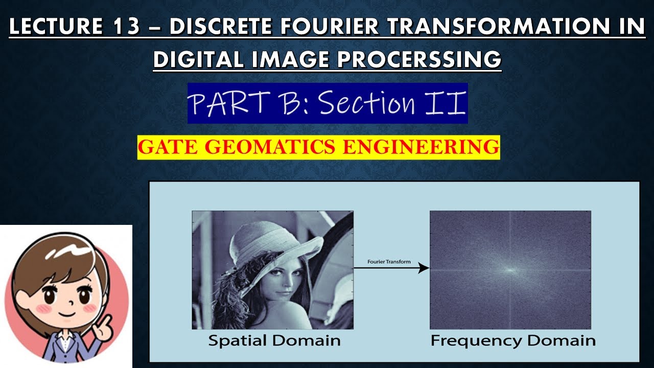
LECTURE 13 - FOURIER TRANSFORMATION IN DIGITAL IMAGE PROCESSING | GATE GEOMATICS ENGINEERING | #gate

Image Formation - II

OpenCV on Google Colab - Working with Gray Image

Pertemuan 2: Citra Digital, Sampling, dan Quantization-Part 5: Konsep dasar Sampling & Quantization
5.0 / 5 (0 votes)
