Normal Data Analysis with Software Part 1
Summary
TLDRIn this tutorial, Matt demonstrates how to use statistical software, specifically StatKey and Statcato, to analyze normal quantitative data. Using a dataset of wrist circumferences from 40 women, he walks through the steps of importing data, calculating descriptive statistics like mean and standard deviation, and visualizing data through histograms and dot plots. The lesson emphasizes identifying normally distributed data, explaining the importance of the mean and standard deviation, and ensuring that the data is bell-shaped for accurate analysis. This video provides a hands-on guide for effective data analysis without manual calculations.
Takeaways
- 📊 The video introduces how to use software to analyze normal quantitative data, specifically focusing on using the mean and standard deviation.
- 💻 The speaker emphasizes the importance of using software to handle calculations, rather than doing them by hand.
- 📈 The dataset used for the analysis is health data, focusing on the wrist circumference of 40 randomly selected women, measured in inches.
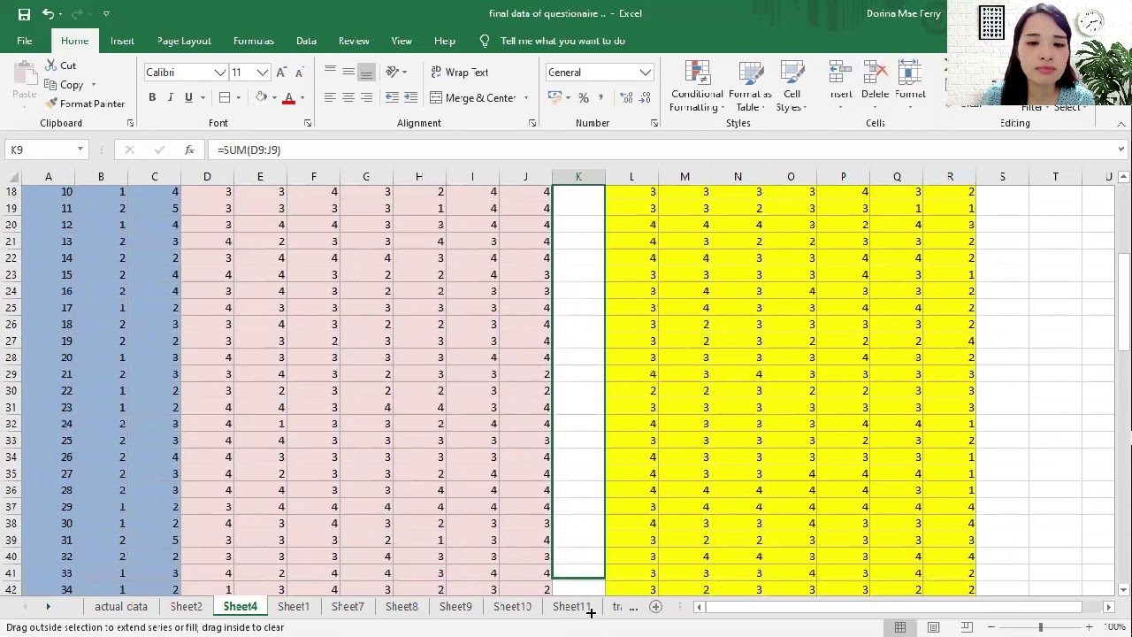
- 🔢 The speaker demonstrates how to copy the data from an Excel file and paste it into analysis software for processing.
- 🖱️ StatKey is the first tool used to calculate the mean (5.067) and standard deviation (0.331) of the wrist circumference data.
- 📐 The importance of checking the shape of the data is highlighted, and a histogram is generated to confirm the data has a normal distribution.
- 📉 The speaker reduces the number of bins in the histogram to better visualize the normal distribution, which is bell-shaped with symmetry on both sides.
- 📊 A comparison between the mean and median is made to confirm that the data is not skewed, as they are close in value.
- 📋 The second software, Statcato, is introduced, and similar calculations (mean and standard deviation) are performed using the same data.
- 📏 The speaker explains that the mean plus or minus one standard deviation captures about 68% of the data, showing the typical range of wrist circumferences in this dataset.
Q & A
What type of data is being analyzed in the video?
-The video analyzes normal quantitative data, specifically focusing on the wrist circumference of 40 randomly selected women, measured in inches.
Why is software used to calculate the mean and standard deviation?
-Software is used to calculate the mean and standard deviation to avoid manual calculation errors and speed up the process, especially when working with large datasets.
What software tools are demonstrated in the video for data analysis?
-The video demonstrates the use of two tools: StatKey and StatCato for calculating descriptive statistics like the mean and standard deviation, as well as creating histograms and dot plots.
How does the presenter suggest pasting data into StatKey?
-The presenter suggests clicking 'Edit Data' in StatKey, deleting any existing data using Ctrl+A (or Command+A on a Mac), and then pasting the new data with Ctrl+V (or Command+V).
What steps are recommended for checking if data is normally distributed?
-To check for normal distribution, the presenter recommends creating a dot plot or histogram in StatKey or StatCato, and adjusting the number of bars (or bins) to ensure the highest bar is in the middle and the tails are symmetric.
What does the mean and standard deviation represent in the context of this dataset?
-The mean (5.067 inches) represents the average wrist circumference of the women in the sample, while the standard deviation (0.331) indicates the spread of the wrist circumference values around the mean.
Why is it important to assess the shape of the dataset before using the mean?
-It is important to assess the shape of the dataset to ensure it is normally distributed, as the mean is only an accurate measure of central tendency when the data follows a normal or bell-shaped distribution.
What additional statistics can be calculated using StatCato?
-In addition to the mean and standard deviation, StatCato can calculate other statistics like the minimum, maximum, median, and sample size (n).
What is the significance of the mean and median being close to each other?
-When the mean and median are close to each other, it suggests that the data is symmetric and not skewed, indicating that the mean is a reliable measure of central tendency.
How does the video demonstrate calculating the range of typical values?
-The video demonstrates calculating the range of typical values by adding and subtracting the standard deviation from the mean. This range (4.736 to 5.398 inches) represents the central 68% of the data, which is typical for normally distributed data.
Outlines
💻 Introduction to Analyzing Quantitative Data with Software
In this section, Matt introduces the topic of using software to analyze normal quantitative data, focusing on why it is more efficient to use computer programs rather than manual calculations. He provides an example using health data from his website, which includes various statistics like age, height, and wrist circumference for 40 men and 40 women. Matt walks through the process of selecting the 'women’s wrist circumference' data from an Excel file, copying it, and preparing it for analysis using statistical software tools like StatKey.
📊 Understanding Data Shape and Normality
Here, Matt explains the importance of knowing the shape of the data to determine if the mean and standard deviation can be used effectively. He discusses how to visually inspect the data's normality using histograms and dot plots. Matt demonstrates adjusting the number of histogram bins (called 'buckets' in StatKey) and explains how the highest bar in the middle and symmetry in the tails signify a normal, bell-shaped distribution, which justifies using the mean and standard deviation.
🔢 Calculating Basic Statistics with StatKey and StatCato
In this paragraph, Matt compares the use of StatKey and StatCato for calculating statistics like mean and standard deviation. He walks through how to paste the wrist circumference data into both tools, explaining how to manipulate columns and bins in StatCato. He reiterates that fewer bins (around three or five) are better for small data sets, and both tools show a normal data distribution. He highlights how the close proximity of the mean and median is a strong indicator of normality.
📐 Using Statistical Tools to Calculate and Interpret Data
Matt discusses the process of finding essential statistics, such as the mean, standard deviation, minimum, maximum, and sample size (n), using the statistics menu in StatCato. He demonstrates how these values are important for understanding the data, emphasizing how adding and subtracting the standard deviation from the mean can reveal 'typical values' that represent 68% of the data. Finally, he organizes the wrist data in ascending order and identifies typical values to further analyze the dataset visually.
Mindmap
Keywords
💡Quantitative Data
💡Mean
💡Standard Deviation
💡Normal Distribution
💡Histogram
💡Dot Plot
💡StatKey
💡Statcato
💡Descriptive Statistics
💡Sample Size
Highlights
Introduction to using software for analyzing normal quantitative data.
Focus on not calculating mean and standard deviation by hand, but rather using computer programs.
Example data set used: health data from 40 women and 40 men, including age, height, and weight.
Specific analysis on women's wrist circumference data in inches.
Emphasized the importance of not altering raw data; advised copying data into new sheets for analysis.
Use of StatKey software to calculate the mean and standard deviation from pasted data.
Initial results: mean wrist circumference is 5.067 inches, and standard deviation is 0.331 inches.
Understanding data shape: importance of normal or bell-shaped distribution to validate the use of mean and standard deviation.
Visualizing data using histograms in StatKey to confirm a normal distribution.
Tips for adjusting histogram bars (bins) in StatKey to better represent small data sets.
Discussion on identifying normal distribution based on symmetrical histogram with the highest bar in the middle.
Comparison between mean and median to further assess data normality.
Use of Statcato software to visualize data and calculate descriptive statistics like mean, standard deviation, and sample size.
Explanation of how mean and standard deviation give typical data values and how to calculate these typical values.
Final data insights: values between 4.736 and 5.398 inches are considered typical for wrist circumference.
Transcripts
hi everyone this is Matt to show with
intro stats and today we're going to
look how to use software to analyze
normal quantitative data so we've kind
of seen the theory behind that we've
seen that we want to use the mean and
the standard deviation when the data
looks normal
but again we actually don't want to
calculate this stuff by hand we want to
actually have a computer program
calculate do the heavy lifting for us so
let's take a look at an example so this
again is my website Matt - to show our G
and we need some data so I'm going to go
to the statistics tab and I'm going to
click on data sets the data we're going
to look at today is the health data this
has here's the health data so I'm gonna
look here it's right here health data
I'm just gonna open the excel file so
health data Excel and you're gonna get
this one now this data actually has a
lot of data it has the random sample
data from 40 women and 40 men so it has
the data separated so you can see the
men's ages and heights and weights and
women's ages and Heights and weights and
things like that and it also has the
combined data so the combined data has
all 80 of the men and women so it does
have quite a beautiful day to set so
when you're looking for something just
keep kind of scrolling to the right
until you find what you're looking for
the data I'm going to look at today is
women's wrist circumference and infor in
inches so the they looked at they
measured how far around the wrist is for
these 40 randomly selected women in
inches okay
so again whenever you're working with
data like don't it's not as a good idea
don't mess up some raw data so I'm just
gonna copy this we learned last time
that if you want you hold your cursor
above the column so it turns into a
downward arrow and then just left-click
and it'll highlight the entire column
for you
and then push control-c or its command
see if you're in a mac and then we're
going to go ahead and paste that into a
new data set here so we have a new data
set here
there we go it's right there there's the
new data set yeah if I want to have the
computer calculate I'm going to use stat
Cato and stat key to calculate the mean
and standard deviation so we'll start
with we'll start with looking at stat
key so again you go to lock 5s com
that's where stat key is hosted you
don't need to save it it works so you
can just open it click on the stat key
button now this was one quantitative
data set so we're gonna click on one
quantitative variable it's under the
descriptive statistics and graphs sort
of on the top left it says one
quantitative variable so we click on
that now whenever you're pasting data
into something into a into stat key
usually you're gonna click the edit data
button so edit data now right now this
is kind of looks kind of weird you'll
notice you'll see the the numbers the
quantitative data but it also has a word
next to every number that sometimes
called an identifier these were how long
do certain animals live in years and
they were kind of showing what animal
that that number came from that's called
an identifier most of my data sets don't
have an identifier necessarily so so
what you're gonna do I'm gonna do is
just delete out this data again an easy
way to delete data out you can click and
drag it down if you want but I just like
push ctrl a ctrl a will highlight
everything even if you got a really huge
data set and then just push delete so
ctrl a delete
now I want to paste in the data that the
wrist data from the 40 randomly selected
women so I'm going to do that now if you
look this data does have a title so
titled means header row in stat in stat
key so you leave this checked it says
header row but it does not have an
identifier it doesn't have a word next
to every number so you want to uncheck
that one and then just push OK and there
we go
if you notice right away it calculated
there was 40 women that's the sample
size we see the mean was 5.0 six seven
we see the standard deviation is 0.33
one but again we have to know we we have
to know two what the shape of this data
set looks like for it to be for us to
know if we can use the mean and standard
deviation so what we said was it needed
to be normal or bell-shaped we can kind
of see from the dot plot that it does
sort of look sort of normal we got more
dots in the middle and as we get away
from the middle we have fewer and fewer
dots but it's better to look at the
histogram let's take a look at the
histogram now the the number of bars is
a lot for a data set is so small we only
have 40 women in this data set so having
10 bars or 10 bins or a stat key calls
it buckets so 10 buckets is a lot of a
lot of bars for this for this small of a
data set so I like to decrease the
amount of buckets you can kind of play
around with this a little bit and have
these go back and forth a little bit but
you can see right away that that looks
pretty normal right you can kind of see
how the data looks looks very normal and
also the mean which is the average 5.0
67 is pretty close to the highest bar
it's sort of right on the highest bar so
this is what we call normal or
bell-shaped the highest bar is in the
middle and the left tail is about
symmetric with the right tail all right
that's though you know normal when you
see it you can also decrease the number
of buckets if you want a number of bins
with this slider so here's here's five
bars or even three bars three bars works
pretty well
especially if the data is very very
small but this thing this data set
looked normal even at five bars or even
at seven bars so it looks pretty normal
we got we definitely have the highest
bar in the middle and it looks pretty
symmetric so we this is normal and what
we learned in our theory is that that's
when the only time the mean actually is
an accurate average so that we are
allowed to use the mean one thing to
take take a look at is that the mean and
the median are actually very close in
when we get to our discussions about
skewed data the the mean sort of gets
pulled in the direction of the skew but
if the mean and the median are actually
very close that's usually a good sign
that you're probably the mean is is
somewhat of an accurate average also
standard deviation is going to be our
spread for normal data okay so we know
the mean is five point zero six seven
and the standard deviation is 0.33 one
now I could have actually found this on
on statcato as well so whenever you're
copying and pasting in stat kado you
always want to make sure the title again
is in the gray so I'm gonna paste in
that data there it is women's wrists
data by the way you can pull these if
you put the cursor in between where it
says c1 and c2 you'll see it turns into
a sideways double arrow if you click you
can drag it open and see the title
better if you want okay so let's take a
look at our graph if we want to graph
this and see what the shape is I would
go graph and histogram all right there's
our histogram and then you just click on
the column that you want to make a graph
of this button down here this is show
legend is a good button it puts a title
on it for you so it's just kind of nice
I always like my graphs tab titles and
number of bins I know a stat key called
them buckets
yes but stat kado calls them bins and so
the number of bins 10 is quite a few I
think I'm gonna decrease this I think we
even like three bars would probably be
pretty well or
five or seven three usually works pretty
well if you have a small small data set
and we can see it does look normal right
the highest bar is definitely in the
middle so it looks looks pretty
symmetric okay and we can also have a
dot plot if we want it so graph and dot
plot and just click on that on the
column you want again show legend we'll
put a title and there's our dot plot so
you can kind of see even the dot plot
looks kind of normal
alright and now how do we find
statistics on stat kado well it's under
the statistics menu so you go to
statistics basic statistics descriptive
statistics
so again statistics basic statistics
descriptive statistics if you just want
to kind of calculate some basic
statistics for a quantitative data set
that's where you'd look again it will
ask you input variable that wants the
column so sometimes it'll have like a
you know you can click on the column but
this one doesn't so we have to type it
in c1 stands for column one so it's the
one that says here it's asking what
variable what column your data is in and
notice you have all kinds of different
statistics that they will calculate
here's a few that are I think are
important especially if you already know
that what I what I always do is find the
shape first and then identify which of
these statistics I want based on the
shape since we already know this data
was normal we're gonna want the mean and
the standard deviation so that they're
the meanest standard deviation right
there also it's nice to have the min and
the max I'd like to know the min and the
max cuz those might be outliers and I
also like to know how many numbers there
were so I like this button this is n
total if you remember the letter n
stands for sample size or how many
numbers are in your data set so those
when I have a normal data set these are
sort of the statistics I like to find
and I just pushed ok and there we go
it calculated it for us notice it got
the same really the same numbers that
stat key gave us the mean was 5.0 6 7
and the standard deviation is 0.33 one
the men was 4.2 max 5.8 and the end
total we had 40 women in the dataset
now what I want to show you though is
what are these numbers mean in terms of
the theory we learned last time so last
time we learned that if you add and
subtract the mean and the standard
deviation you get the typical values the
typical values so five point zero six
seven the mean minus 0.33 one the
standard deviation gives us four point
seven three six and the mean plus the
standard deviation gives us five point
three nine eight if you remember last
time where I mentioned that that's about
the middle 68% of the data now I just
want to kind of show you where that
sounds oh it's good to kind of have a
visual of the data now the one thing
about this is again this data is not in
order so what I'd like to do is just
kind of put it in order so I'm gonna
highlight this data set I'm gonna go to
home and right here you'll see sort sort
and I'm gonna sort smallest to largest
there we go and that just makes it
easier for me to kind of see this
visually so anything between four point
seven three six so four point seven
would be less so it has to be between
four point seven three six and five
point three nine eight are going to be
considered typical all right so this
would be considered typical all right so
there's our our four point eight
Voir Plus de Vidéos Connexes
The Empirical Rule
Descriptive Statistics: FULL Tutorial - Mean, Median, Mode, Variance & SD (With Examples)
03 Descriptive Statistics and z Scores in SPSS – SPSS for Beginners
Quantitative Data Analysis 101 Tutorial: Descriptive vs Inferential Statistics (With Examples)
4. Grade 11 Mathematics - Statistics - Standard Deviation Calculations
Como calcular assimetria dos valores no Azure SQL Server
5.0 / 5 (0 votes)