This Downward Pointing Triangle Means Grad Div and Curl in Vector Calculus (Nabla / Del) by Parth G

Summary

This video introduces important differential operators—gradient, divergence, and curl—commonly used in physics and vector calculus. It explains how the 'nabla' operator is applied to scalar and vector fields, demonstrating how these operators measure changes in different directions. Through clear examples, such as flour distribution and fluid flow, the video delves into the concepts of gradient (change in a scalar field), divergence (outflow or inflow of a vector field), and curl (rotation in a vector field). The speaker also links these concepts to Maxwell's equations in electromagnetism.

Takeaways

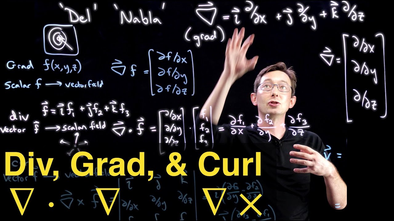
• 🔺 Nabla (or del) is a vector used to represent differential operators like gradient, divergence, and curl.
• 🔄 Gradient measures how quickly a scalar field changes in space and results in a vector field.
• 📏 Partial derivatives (denoted by ∂) help isolate the change in a specific direction while keeping others constant.
• 🌍 Scalar fields represent quantities like altitude or temperature, and the gradient of these fields indicates the direction of the steepest ascent.
• 🌬️ Vector fields can represent physical phenomena like wind or electric fields, assigning a vector to each point in space.
• ⚡ Divergence measures how much a vector field spreads out from a point and can indicate sources or sinks in fields like electric fields.
• 💥 In electromagnetism, the divergence of an electric field relates to the presence of electric charges, and divergence of magnetic fields is always zero (no magnetic monopoles).
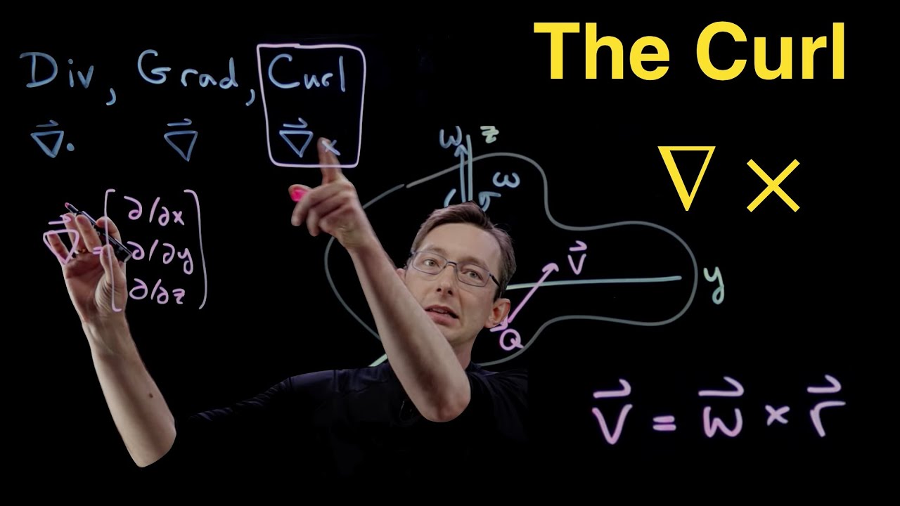
• 🔁 Curl measures the rotation or circulation of a vector field, such as the rotation of fluid flow, and results in another vector field.
• 📐 In physics, the curl operator is used in Maxwell’s equations, showing how changing magnetic fields induce electric fields.
• 🎓 Gradient, divergence, and curl are essential tools in vector calculus, with applications in physics like gravity, electromagnetism, and fluid dynamics.

Q & A

What are the gradient, divergence, and curl operators, and where are they commonly used?

The gradient, divergence, and curl operators (often called grad, div, and curl) are differential operators used in vector calculus. They are widely used in physics, particularly in areas like fluid dynamics, electromagnetism, and gravitational fields. The gradient measures the rate of change of a scalar field, the divergence measures how much a vector field spreads out from a point, and the curl measures the rotation or circulation of a vector field.

What is the del (nabla) operator, and how does it relate to partial derivatives?

The del (nabla) operator, denoted by a downward-pointing triangle, acts like a vector of partial derivatives in three dimensions. Its components are partial derivatives with respect to x, y, and z. It measures how quickly a quantity changes over small distances in different directions.

How does the gradient operator work, and what does it represent?

The gradient operator, when applied to a scalar field, gives a vector field that represents the direction and rate of fastest change of the scalar field. For example, in a topographical map, the gradient would indicate the direction of the steepest incline at each point.

What is the physical interpretation of the divergence of a vector field?

The divergence of a vector field gives a scalar value that represents how much the field is spreading out or converging at a point. For instance, in fluid flow, a positive divergence would indicate that fluid is flowing out from a point (a source), while a negative divergence indicates fluid flowing into a point (a sink).

How does the curl operator work, and what does it measure?

The curl operator, when applied to a vector field, produces another vector field that represents the rotation or circulation of the original vector field. The direction of the resulting vector indicates the axis of rotation, while the magnitude represents the strength of the rotation.

Can you explain the physical significance of scalar and vector fields?

A scalar field assigns a single value to each point in space (e.g., temperature distribution), while a vector field assigns a vector to each point (e.g., wind speed and direction). Scalar fields measure quantities like height or temperature, while vector fields measure directional phenomena like electric fields or fluid flow.

How is the gradient of a scalar field applied in physics, particularly with gravitational fields?

In physics, the gradient of a scalar field, such as the gravitational potential, gives a vector field representing the gravitational force. The direction of the gradient indicates the direction in which the gravitational force acts, while its magnitude shows the strength of the force.

What role does the dot product play in calculating divergence?

The dot product in the context of divergence applies the del operator to a vector field. It combines the partial derivatives from the del operator with the components of the vector field, resulting in a scalar field that measures how much the field is expanding or contracting at a point.

How are Maxwell's equations related to the divergence and curl operators?

Maxwell's equations, which describe electric and magnetic fields, make extensive use of divergence and curl. For example, one of the equations states that the divergence of the magnetic field is always zero, implying no magnetic monopoles exist. Another equation involves the curl of the electric field, which is related to the changing magnetic field over time.

What is the difference between applying the gradient, divergence, and curl to fields in vector calculus?

The gradient is applied to a scalar field and results in a vector field, representing the direction of steepest change. The divergence is applied to a vector field and results in a scalar field, representing how much the field spreads out from a point. The curl is applied to a vector field and results in another vector field, representing the rotation or circulation of the original field.

Outlines

00:00

🔍 Introduction to Differential Operators: Grad, Div, and Curl

In this paragraph, the speaker introduces three important differential operators—gradient, divergence, and curl—commonly abbreviated as grad, div, and curl. These operators are frequently used in physics and other fields. The speaker explains that the video will first clarify the meaning of each operator and then explore their applications.

05:01

🔺 Understanding the Nabla Operator (Del)

This paragraph introduces the nabla or del operator, represented by a downward-pointing triangle. Del acts as a vector in three dimensions with partial derivatives along the x, y, and z axes. It measures how a quantity changes over small distances in different directions. The speaker also notes that del is essential for understanding the grad, div, and curl operators and is part of vector calculus.

10:02

🌸 Example: Applying the Del Operator to a Flour Distribution

Using the example of a flour packet being squished, the speaker explains how the del operator is applied. The flour distribution, denoted as 'f,' is analyzed by taking the partial derivative with respect to x, dx. The resulting value indicates how quickly the distribution changes along the x-axis. The speaker emphasizes that partial derivatives represent changes in one direction while keeping other variables constant.

📏 Scalar Fields and Gradient of a Scalar Field

This section dives deeper into scalar fields, which assign values to points in space, such as altitude on a map. By applying the del operator to a scalar field, one obtains a vector field, which represents the rate and direction of the fastest change at each point. The speaker uses a height map to illustrate this concept, where vectors point in the direction of steepest ascent.

🌬️ Vector Fields: Gradient, Wind, and Electric Fields

Here, the speaker explains vector fields, which assign vectors (rather than scalar values) to each point in space. Examples include the direction of wind flow or the electric field created by charged particles. The divergence of a vector field is introduced, showing how it measures the net amount of field entering or leaving a region, with electric fields obeying specific rules from Maxwell's equations.

🔄 Curl: Measuring the Rotation of Vector Fields

The curl of a vector field is introduced as a measure of its circulation or rotation. Using a water flow example, the speaker explains how a fan dropped into flowing water would rotate, with the curl operator representing this rotation as a new vector field. The direction and magnitude of the resulting vector describe the axis and strength of the rotation.

🔗 Applications of Grad, Div, and Curl in Physics

This paragraph highlights the application of grad, div, and curl in physics. The gradient of a scalar field can represent a gravitational field, while Maxwell's equations link the divergence of the electric field and the curl of the magnetic field. These operators help explain intricate relationships between electric, magnetic, and gravitational fields.

👋 Conclusion and Call to Action

In the concluding paragraph, the speaker wraps up the video, thanking viewers for watching and encouraging them to like, subscribe, and support the channel through Patreon. The speaker also mentions other related videos for those interested in further exploration of the discussed topics.

Keywords

💡Gradient (Grad)

The gradient, often denoted as 'grad', measures how a scalar field changes in space. It points in the direction of the steepest ascent of a function and gives the rate of change in that direction. In the video, it is used to explain how quantities like altitude or flour distribution change over space, where the gradient at each point shows the direction and magnitude of the fastest increase.

💡Divergence (Div)

Divergence, symbolized as 'div', measures how much a vector field spreads out from a point. A positive divergence indicates that vectors are 'diverging' or moving outward from a source, while a negative divergence shows convergence. In the video, it is used to describe how electric fields behave around charges, where field lines spread out from positive charges and converge at negative charges.

💡Curl

Curl is a vector operator that measures the rotational tendency of a vector field. It indicates how much and in what direction the field 'curls' around a point. The video explains curl in terms of fluid flow, illustrating how it can show the rotation of particles in a fluid, and relates it to the behavior of magnetic fields.

💡Nabla (Del) Operator

The nabla or 'del' operator (∇) is a mathematical symbol used in vector calculus to calculate gradient, divergence, and curl. It acts as a vector of partial derivatives. In the video, it's shown as a versatile tool for analyzing how fields (scalar or vector) change across space, helping to compute both gradients and how much fields are spreading (divergence) or rotating (curl).

💡Scalar Field

A scalar field is a mathematical function that assigns a scalar (a single value) to every point in space. In the video, examples like altitude or the distribution of flour are used to illustrate scalar fields. The gradient of a scalar field gives a vector field showing the direction and rate of fastest increase at each point.

💡Vector Field

A vector field assigns a vector to every point in space, describing quantities like velocity or electric field. The video uses examples like wind flow and electric fields to explain vector fields. For instance, in an electric field, the vectors show the force experienced by a charged particle at each point in space.

💡Partial Derivative

A partial derivative represents the rate of change of a function with respect to one variable while keeping other variables constant. The video explains partial derivatives in terms of flour distribution across the x, y, and z directions, illustrating how the change in one direction is isolated.

💡Dot Product

The dot product is a mathematical operation that multiplies two vectors to produce a scalar. In the video, it's used to describe how divergence is calculated by taking the dot product of the del operator with a vector field, giving a scalar field that shows the amount of field spreading or converging at each point.

💡Cross Product

The cross product is a vector operation that produces a third vector perpendicular to two given vectors, representing their mutual rotation or circulation. The video uses the cross product to explain curl, showing how it measures the rotational tendency of a vector field like fluid flow or magnetic fields.

💡Maxwell's Equations

Maxwell's equations are fundamental laws of electromagnetism that describe how electric and magnetic fields behave. In the video, these equations are referenced to show the divergence and curl of electric and magnetic fields, such as how the curl of the electric field relates to the changing magnetic field, demonstrating the deep connection between electricity and magnetism.

Highlights

Introduction of the key differential operators: Gradient, Divergence, and Curl, often shortened to Grad, Div, and Curl, which are essential in physics and other fields.

Explanation of the nabla (∇) or del operator, which acts as a vector with components representing partial derivatives in three dimensions (d/dx, d/dy, d/dz).

Clarification that ∇ can be applied to scalar or vector fields to measure the rate of change in different directions, linking vector calculus and physics.

Demonstration of gradient (grad) by applying ∇ to a scalar field to find how fast the quantity changes at each point, resulting in a vector field.

Explanation of divergence (div) as the dot product of ∇ and a vector field, measuring the net flow of a vector field, leading to a scalar field.

Illustration of how the divergence of the electric field shows whether the field originates from a source (positive charge) or a sink (negative charge).

Description of curl as the cross product of ∇ and a vector field, measuring the rotational motion or circulation at each point, resulting in another vector field.

Visualization of curl by imagining water flow and a fan placed in it, with the fan’s rotation representing the vector field’s curl.

Notion that scalar fields can represent real-world quantities like altitude or a distribution of flour in space, helping to visualize grad, div, and curl concepts.

Connection between grad and the gravitational field, with the gradient of gravitational potential φ resulting in the gravitational field, explained with negative sign convention.

Application of div in Maxwell’s equations, showing how the divergence of the magnetic field is always zero, indicating no isolated magnetic poles.

Curl’s role in Maxwell’s equations, where the curl of the electric field is linked to the time rate of change of the magnetic field, reinforcing the deep connection between electric and magnetic fields.

Explanation of scalar and vector fields: Scalar fields assign a single value at each point, while vector fields assign a direction and magnitude.

Visual example of the gradient of a scalar field using a height map, where the vectors point toward the direction of the steepest increase.

Final notes on the applications of grad, div, and curl in physics, particularly in electromagnetism and gravitational theory, illustrating the operators’ widespread use in theoretical and applied contexts.

Transcripts

hey everyone parth here and in this

video we will be looking at an

important group of differential

operators known as gradient divergence

and curl

these are often shortened to grad div

and curl and they're used very regularly

in the world of physics as well as

elsewhere

so we'll start by understanding what

each one of these actually means and

then we'll be looking at some

applications

to understand the grad div and curl

operators we need to start by thinking

about this downward pointing triangle

known as the nabla or del del can be

thought of as a vector

in three dimensions it looks something

like this the components of the vector

are partial derivative d by d

x partial derivative d by d y and

partial derivative d by d

z each one of these measures essentially

how quickly a particular quantity

changes

over a small distance in the x direction

y direction and z direction

now if you've seen my recent poisson

equation video and you're familiar with

partial derivatives as well as

del then feel free to skip to this

timestamp here so let's take a more

detailed look at dell

now for example if we've got a packet of

flour and we open this packet and we

decide to squish it

so the flour goes everywhere and then we

plot how much flour is found at every

point along

the x direction we can see that our

flour distribution would look something

like this lots of flower near the origin

and then less and less the further we

get away from the origin

let's also say that we label this flower

distribution as f

and let's now try and find df by dx this

simply measures how quickly our flower

distribution changes

as we move along the x-axis we can think

of this as measuring the gradient or

slope

of our flower distribution function over

here for example our flower distribution

drops off very quickly so the gradient

is steep

and hence df by dx has a large size and

of course is negative because the flower

is decreasing

whereas in this region the amount of

flower is not changing a huge amount

therefore the gradient is shallow and df

by dx has a small

magnitude and is again negative because

the flower is decreasing as we move from

left to right

basically d by dx of our flower

distribution f

is simply measuring how quickly the

flower distribution changes

now we could apply this nabla operator

to our function

f and we would get in the first instance

df by dx as we've already seen

except the nabla operator has these

weird curly d's

they're not normal d's now as it turns

out these curly d's are representing

what's known as a partial

derivative and luckily these are fairly

simple to think about at least in a

basic way

if we realize that our flower

distribution for example doesn't just

vary over the x direction

but it also varies in other directions

for example the y direction then we can

understand that the curly d's in df by

dx

mean that we're only measuring the

change in the x direction whilst keeping

everything else constant

similarly the curly df by dy isolates

out the change in the flower

distribution in the y direction

whilst keeping everything else constant

so we're not having to worry about the

change in the x direction

anyway so that's what dell ends up

representing and as we've already seen

this is what dell looks like in three

dimensions if we're only working in two

dimensions then del would look like this

and so on we'll notice that del is a

vector and it contains partial

derivatives which are studied in

calculus and hence del

is an operator in the area of

mathematics known as vector calculus but

we keep saying this word

operator what does it actually mean well

the nabla operator

can operate on or do stuff to certain

mathematical entities in this case

scalar fields or vector fields a scalar

field is basically a field of numbers or

values

in other words every point in a given

space whether that's real space or some

abstract space that we're considering

can be assigned a value

we can use scalar fields to represent

things like altitude on a map

in this particular case we're using it

to represent how high above sea level

you would be

if you were to stand on that point of

the earth or it could be used to

represent the amount of flour found in a

given region of space

after we'd squished our bag of flour and

of course those are just two of the more

physical examples see if you can come up

with your own example of how we can use

scalar fields

now the del operator can be used to find

out how quickly our scalar field changes

at

every point in other words we can find

the gradient of the scalar field

let's stick with our height above

c-level example from earlier

by applying the del operator to our

scalar field

h we get something like this the diagram

shows the gradient

of our scalar field h at each point we

see that there is an arrow or a vector

and each vector points in the direction

that the scalar field

increases most quickly so for example if

our scalar field looks something like

this

and we focus in on the point in the

middle then we can see that the scalar

field increases most quickly

in this direction so in our diagram of

the gradient of our field f

we would get a vector pointing in that

direction and of course the size or

magnitude of that vector

represents exactly how much our scalar

field is changing

so the crux of the matter is that

applying our nebula operator to a scalar

field

gives us a vector field that represents

the rate and direction

of fastest change of our original scalar

field

by the way a vector field is just a

field where we can assign a vector to

every point in that space

and in this case we can see that the

gradient of a scalar field will end up

being a vector field

however a vector field is not always

restricted to just being the gradient of

a scalar field

we can have other vector fields that

aren't necessarily the gradient of a

scalar field too

for example we can think of a vector

field that represents the direction in

which

wind is flowing the direction of each

vector tells us the direction in which

air particles are moving at that point

in space

and the magnitude or size of the vector

tells us how quickly they're moving the

speed of the particles

also in physics we can use a vector

field to represent the electric field

created by charged particles which

actually represents the following

if we were to take a small positively

charged particle and place it at a

particular point in the electric field

then the field lines tell us the size

and direction of the force

that that positive charge would

experience now here's something

interesting we can find out about every

vector field let's imagine that we think

of some imaginary sphere

in this region of space we can measure

exactly how much electric field

enters our sphere and equally we can

measure exactly how much electric field

leaves our imaginary sphere here we see

a certain number of

long arrows entering our sphere which

means that a certain amount of electric

field is entering our sphere or at least

we can imagine it that way

and on the other side we see a lot more

smaller

electric field lines leaving the sphere

and it turns out that for electric

fields specifically

it is always true that the amount of

electric field entering our imaginary

surface

has to equal the amount of electric

field leaving our imaginary surface

the amount coming in always has to

balance out exactly the amount going out

and this is always true except for when

our imaginary surface

is surrounding a charged particle a

positive charge is known as the source

of an electric field which means that

electric field lines originate from a

positive charge

and if we find a positive electric

charge within our imaginary sphere

then the net effect is that electric

field lines are said to be leaving

the sphere conversely a negative

electric charge is said to be a sink of

electric field lines in that electric

field lines end at negative charges

therefore if a negative charge is found

within our imaginary sphere

then the net effect is that electric

field lines are actually entering our

sphere

and as we've already seen in any other

region where there are no charged

particles within our sphere

the net effect is that the amount coming

in exactly cancels out the amount going

out

the reason that the electric field

behaves in this way is specifically

because of

this maxwell equation if you haven't

seen my video covering this maxwell

equation then check it out up here

now in this maxwell equation we can see

that the del operator

is indeed operating but it's no longer

acting as the gradient operator

and we can see that specifically because

of this little dot in between

the del and the e representing the

electric field

this dot is representing a dot product

or a scalar product

between del and the electric field e for

those of you not familiar with the dot

product between two vectors it's when

you take the corresponding components

from the two vectors

multiply them together and then add up

all these little products

but in this situation where the first

vector is the del

what we actually do is apply the partial

derivative to the corresponding

component of the electric field

and remember that the electric field is

a vector field and what we've just seen

is how to find

the divergence of our electric field

even though we see a del

in this location we're no longer taking

the gradient as we saw earlier with the

scalar field

we're now taking the divergence of the

vector field and that's all

changed simply by this little dot and

when we take the divergence off a vector

field what we end up with

is a scalar field in this particular

case it tells us exactly how much

electric field is entering or leaving a

particular point

and this is slightly different to the

gradient operator from earlier because

the gradient operator is applied to a

scalar field

and gives us a vector field now we've

seen how we can take a dot product

between del

and a vector field and as it turns out

we can also find the cross product

for a moment if we think about two

arbitrary vectors and we try and find

the cross product or the vector product

between them

the end result is usually a third vector

perpendicular to the first two

that is also a measure of how unaligned

the two vectors are and this is what i

mean by that

the size of the vector that we get by

taking the cross product between the

first two vectors

will be as large as possible if the

first two vectors are orthogonal to each

other or at right angles to each other

whereas if the two original vectors are

exactly aligned or exactly anti-aligned

then the vector resulting from the cross

product will have a size of zero

but if we now come back to thinking

about vector fields and del

we can find the cross product between

del and a vector field

and in this case things are slightly

different the cross product also known

as the curl

of the vector field is a measure of the

circulation

of our vector field let's imagine that

our vector field is representing some

sort of fluid flow let's say some water

flowing in like

a lake and in this water we drop some

sort of plastic fan

at every point in our vector field we

can measure the rotation that this fan

would experience

and whether it will rotate clockwise or

anti-clockwise

now we can represent the rotation of our

fan

with another vector that points along

the axis

of rotation a common convention is to

say that if the fan

rotates clockwise then our vector

representation will point

downward and if it rotates

anti-clockwise then it will point up

towards us

and the size or magnitude of this vector

represents the size or magnitude of the

rotation

and this is exactly what we measure when

we apply the curl operator

to our original vector field the end

result is another vector field that

represents the axis of rotation

of each part of the original fluid flow

in this case

it's important to note though that the

rotation is not a property of the fan

it's actually the fluid flow that's

causing our imaginary fan to rotate

and therefore the curl is actually

measuring something about the original

vector field

and so bringing it all the way around we

earlier saw that when we apply gradient

to a scalar field

the end result is a vector field when we

apply divergence to a vector field the

end result is a scalar field

and when we apply curl to a vector field

the end result is a vector field

but it's also important to understand

what each one of these represents

now in physics all three of these

operators are used very regularly

for example the gradient of a scalar

field phi

is directly related to the gravitational

field produced by

some object with mass and in this

particular case the scalar field phi is

known as the gravitational potential

now in this case we've got a negative

sign because the rate of increase of the

gravitational potential

points in the opposite direction to the

gravitational field itself but we can

see the use of the grand operator on a

scalar field in this particular instance

in electromagnetism we've seen that

maxwell's equations deal with electric

and magnetic fields

and we've already seen one of these

equations earlier in the video

but another one tells us that if our

theory of classical electromagnetism is

correct

then the divergence of the magnetic

field is always

zero in other words there are no lone

sources or sinks

of the magnetic field for more

information on this check out my video

on that maxwell equation and finally

another maxwell equation

tells us that the curl of the electric

field is equal to minus the time rate of

change of the magnetic field

in this way we see an intricate link

between electric and magnetic fields and

we see also the use of the curl operator

for more information on that maxwell

equation check out this video up here

and with all of that being said i'm

going to finish up here thank you so

much for watching if you enjoyed the

video please do hit the thumbs up button

and subscribe for more fun physics

content

hit the bell button if you'd like to be

notified when i upload and please do

check out my patreon page if you'd like

to support me on there

thank you as always for your wonderful

support and i will see you very soon

[Music]

you