ECE 461.11 First and Second Order Approximations
Summary
TLDRIn ECE 461 Lecture 11, the focus is on first and second order approximations for control systems. The lecture explains the concept of dominant poles, which are crucial for simplifying high-order systems while preserving their behavior. It covers how to identify these poles and match the DC gain for an accurate model. The importance of settling time, overshoot, and damping ratio is discussed, with methods to determine these parameters from a system's step response. The lecture also touches on the practical use of these concepts in real-world applications, such as car suspensions and missile systems.
Takeaways
- 📚 The lecture introduces first and second order approximations for control systems, emphasizing the impracticality of manually calculating higher order systems like the 250th order Maverick missile model.
- 🔍 The concept of dominant poles is highlighted as crucial in understanding system responses, where one or two poles usually have the most significant impact on the system's behavior.
- 🚗 An example is given using a car's vibrational modes to illustrate how the lump mass of the car represents the dominant pole in its response to road conditions.
- 🔑 The importance of modeling is underscored, with the goal of creating a simpler yet accurate representation of a system by matching the dominant pole and DC gain.
- 📉 Definitions of key terms such as 'dominant pole', 'DC gain', 'two percent settling time', 'overshoot', and 'damping ratio' are provided to establish a foundation for understanding control systems.
- 📈 The process of identifying the dominant pole is explained, often being the pole closest to the origin, and its significance in creating a simplified model of the system.
- 📝 The method of determining system parameters from the step response is demonstrated, showing how the DC gain and settling time can be used to infer the system's characteristics.
- 🔄 The script discusses how to handle complex poles, which require considering both the real and imaginary parts to understand the system's behavior fully.
- 📊 The relationship between the damping ratio and overshoot is detailed, explaining how the damping ratio can be used to predict the system's stability and response to changes.
- 📚 A summary of second order systems is mentioned, which would likely include graphical representations and tables for quick reference in determining system characteristics from response data.
- 🔧 The lecture concludes with an overview of how to use the information about dominant poles and system responses to approximate and understand the behavior of more complex systems.
Q & A
What is the main purpose of identifying dominant poles in control systems?
-The main purpose of identifying dominant poles is to simplify the analysis of a system by focusing on the poles that significantly influence the system's response, allowing for a more manageable and accurate model.
Why is it impractical to find the step response for very high order systems by hand?
-Finding the step response for very high order systems by hand is impractical because it becomes extremely complex and time-consuming, and it can lead to a loss of intuitive understanding of the system's behavior.
What is meant by the term 'DC gain' in the context of control systems?
-The DC gain refers to the gain of a system at low frequencies, specifically at s equals zero, which indicates the system's steady-state response to a constant input.
How is the two percent settling time defined in control systems?
-The two percent settling time is defined as the time it takes for the system's response to reach and stay within 2% of the final steady-state value, which is a standard used for simplicity in calculations.
What is the significance of the damping ratio in control systems?
-The damping ratio is significant as it indicates the amount of overshoot in the system's response to a step input, which is crucial for designing systems with desired stability and performance characteristics.
How can the dominant pole be determined for a system with multiple poles?
-The dominant pole can be determined by analyzing the system's step response or by identifying the pole closest to the origin, as it usually has the largest initial condition and decays the slowest, thus having the most significant impact on the system's response.
What is the relationship between the dominant pole and the system's step response?
-The dominant pole largely dictates the behavior of the system's step response, including the speed of response and the amount of overshoot, making it a key factor in system modeling and analysis.
Why might a simplified model that retains the dominant pole and matches the DC gain be considered 'good enough' for many applications?
-A simplified model that retains the dominant pole and matches the DC gain is considered 'good enough' because it captures the essential behavior of the system, providing an 80-85% accurate representation that is both manageable and useful for most practical purposes.
How can complex poles be handled in the context of system modeling and approximation?
-Complex poles can be handled by ensuring that their complex conjugate is also included in the model, effectively treating them as a second-order system for the purpose of approximation and analysis.
What is the concept of time scaling in control systems, and why is it used?
-Time scaling is the concept of adjusting the time units used in system analysis to align the dominant pole with a more manageable location, typically near minus one, simplifying calculations and making the system's behavior more intuitive.
How can the step response of a system be inferred from its transfer function without explicitly calculating it?
-The step response can be inferred by examining the transfer function's dominant pole and DC gain, as these parameters provide insights into the system's settling time and steady-state behavior, allowing for an estimation of the step response characteristics.
Outlines

Esta sección está disponible solo para usuarios con suscripción. Por favor, mejora tu plan para acceder a esta parte.
Mejorar ahoraMindmap

Esta sección está disponible solo para usuarios con suscripción. Por favor, mejora tu plan para acceder a esta parte.
Mejorar ahoraKeywords

Esta sección está disponible solo para usuarios con suscripción. Por favor, mejora tu plan para acceder a esta parte.
Mejorar ahoraHighlights

Esta sección está disponible solo para usuarios con suscripción. Por favor, mejora tu plan para acceder a esta parte.
Mejorar ahoraTranscripts

Esta sección está disponible solo para usuarios con suscripción. Por favor, mejora tu plan para acceder a esta parte.
Mejorar ahoraVer Más Videos Relacionados
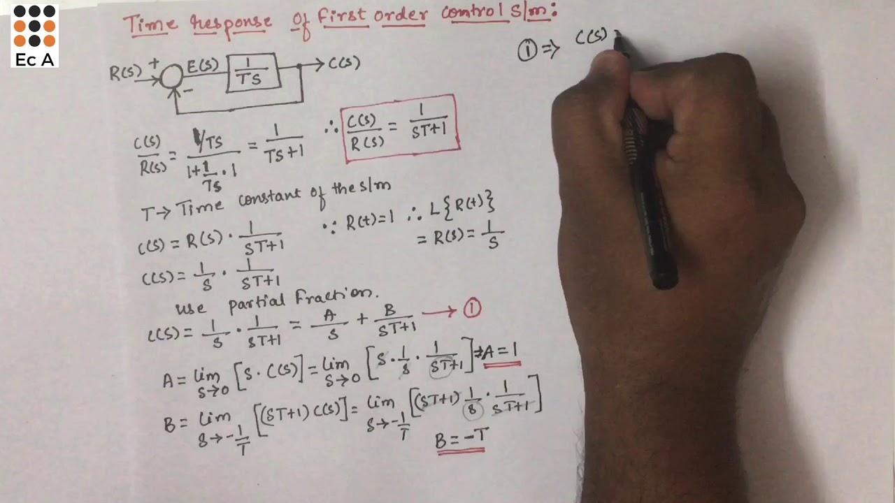
#173 Time response of first order control system || EC Academy

ES2C6 L4c
Lecture: Model-based control design

Sistem Kontrol #3b: Analisis Respon Waktu Sistem Orde 1

#131 Introduction to CONTROL SYSTEMS | open loop and closed loop control system || EC Academy
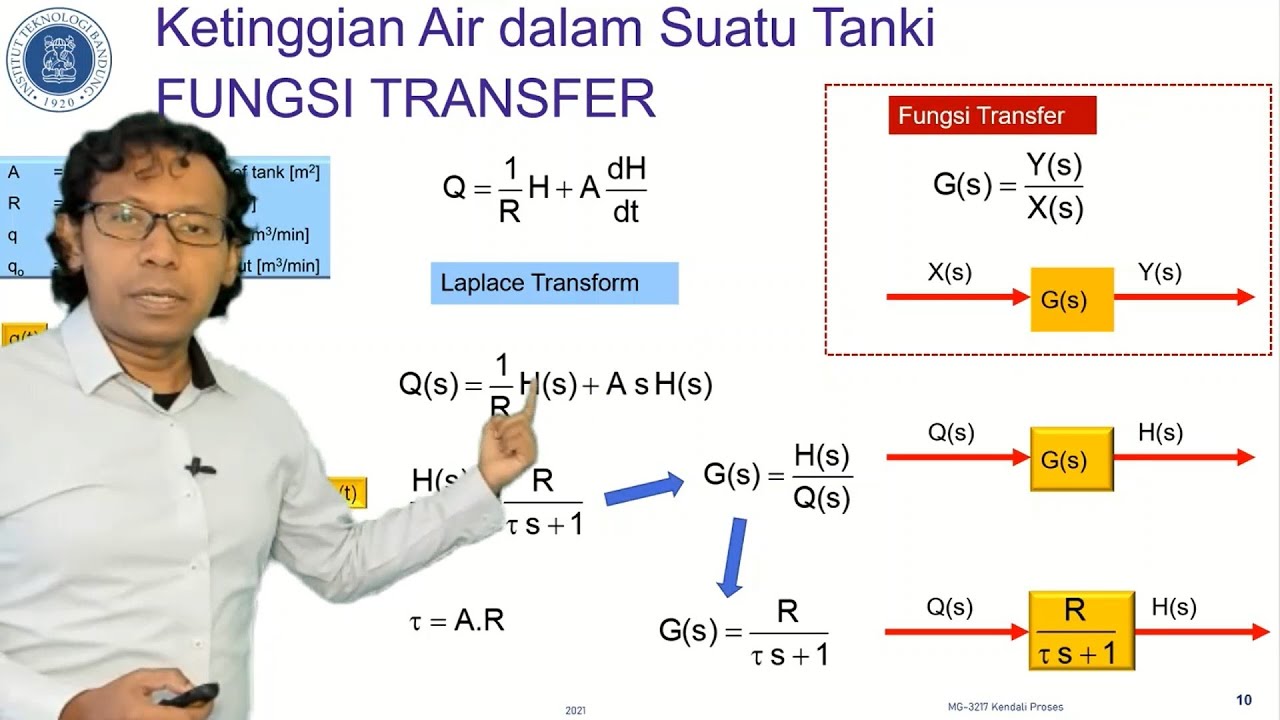
03. MG3217 Kendali Proses S01: Respons Sistem Orde - 1
5.0 / 5 (0 votes)
