Excel GROUPBY & PIVOTBY Functions - All You Need to Know (do they BEAT Pivot Tables? 🤔)
Summary
TLDRThe video introduces two new Excel functions, GROUPBY and PIVOTBY, that provide powerful ways to aggregate, analyze, and present data. It demonstrates how these dynamic functions can automatically group data, calculate totals and subtotals, handle dates, exclude unwanted data, and pivot data from rows into columns. Key benefits over pivot tables include easier filtering, text support, and automatic updates. Overall, these functions enable faster, more flexible Excel reporting while avoiding tedious manual steps.
Takeaways
- 😀 The new GROUPBY and PIVOTBY functions allow for easier data aggregation and pivot table-like reporting directly in Excel formulas
- 😃 GROUPBY has 3 required arguments: Row fields (categories), Values (numbers to aggregate), and Aggregation function like SUM()
- 📈 Optional arguments in GROUPBY: show field headers, toggle totals, sort order, filter array
- 📊 PIVOTBY pivots data with row and column fields for layout; useful when report gets too long
- 📉 GROUPBY can return text values, unlike pivot tables, using functions like ARRAYTOTEXT()
- 🔢 GROUPBY excludes errors and stray calculations, cleaning up the data
- 🗓 GROUPBY can easily handle date fields using the YEAR() and TEXT() functions
- 🤝 HSTACK() helps include multiple fields like dates and categories in GROUPBY rows
- 📌 GROUPBY and PIVOTBY formulas update dynamically when source data changes
- ⬇️ PIVOTBY has additional options to customize column totals, sorting and filtering
Q & A
What are the two new Excel functions introduced in the video?
-The two new Excel functions introduced are GROUPBY and PIVOTBY.
What are the mandatory arguments for the GROUPBY function?
-The mandatory arguments for the GROUPBY function are: Row fields, Values, and Function.
How can you exclude certain rows from aggregations in the GROUPBY function?
-You can use the Filter Array optional argument in GROUPBY to exclude rows based on criteria.
What is one advantage of using GROUPBY over pivot tables?
-One advantage is that GROUPBY results are dynamic - any changes to the source data will automatically update the GROUPBY output.
How can you handle dates in the GROUPBY function?
-Dates can be handled by wrapping them in functions like YEAR or TEXT to extract specific components like year and month.
When would you use PIVOTBY instead of GROUPBY?
-Use PIVOTBY when you want one of the grouping categories in the columns instead of the rows to avoid too much horizontal scrolling.
What are the additional arguments available in PIVOTBY?
-PIVOTBY has a Columns argument to specify which fields should be pivot columns. It also has additional options like Column Total Depth.
Can GROUPBY and PIVOTBY output text fields?
-Yes, by using text aggregation functions like ARRAYTOTEXT or writing a custom Lambda function.
How can the GROUPBY output be sorted?
-The optional Sort Order argument allows sorting the GROUPBY output by a specified column.
What calculations can be used to aggregate values in GROUPBY?
-Options like SUM, AVERAGE, MEDIAN, MAX, MIN, PERCENTOF and custom Lambda functions can be used.
Outlines

Esta sección está disponible solo para usuarios con suscripción. Por favor, mejora tu plan para acceder a esta parte.
Mejorar ahoraMindmap

Esta sección está disponible solo para usuarios con suscripción. Por favor, mejora tu plan para acceder a esta parte.
Mejorar ahoraKeywords

Esta sección está disponible solo para usuarios con suscripción. Por favor, mejora tu plan para acceder a esta parte.
Mejorar ahoraHighlights

Esta sección está disponible solo para usuarios con suscripción. Por favor, mejora tu plan para acceder a esta parte.
Mejorar ahoraTranscripts

Esta sección está disponible solo para usuarios con suscripción. Por favor, mejora tu plan para acceder a esta parte.
Mejorar ahoraVer Más Videos Relacionados

Excel Tutorial for Beginners

Excel Tutorial - What is Excel used for?

16 BELAJAR SQL - FUNGSI AGREGAT / AGGREGATE FUNCTION DI SQL SUM, COUNT, AVG, MIN, MAX
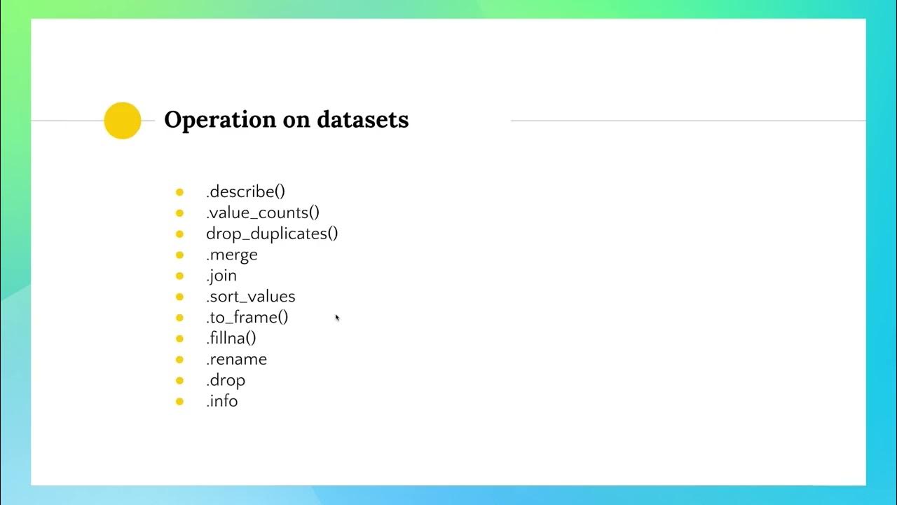
Dataframes Part 02 - 02/03
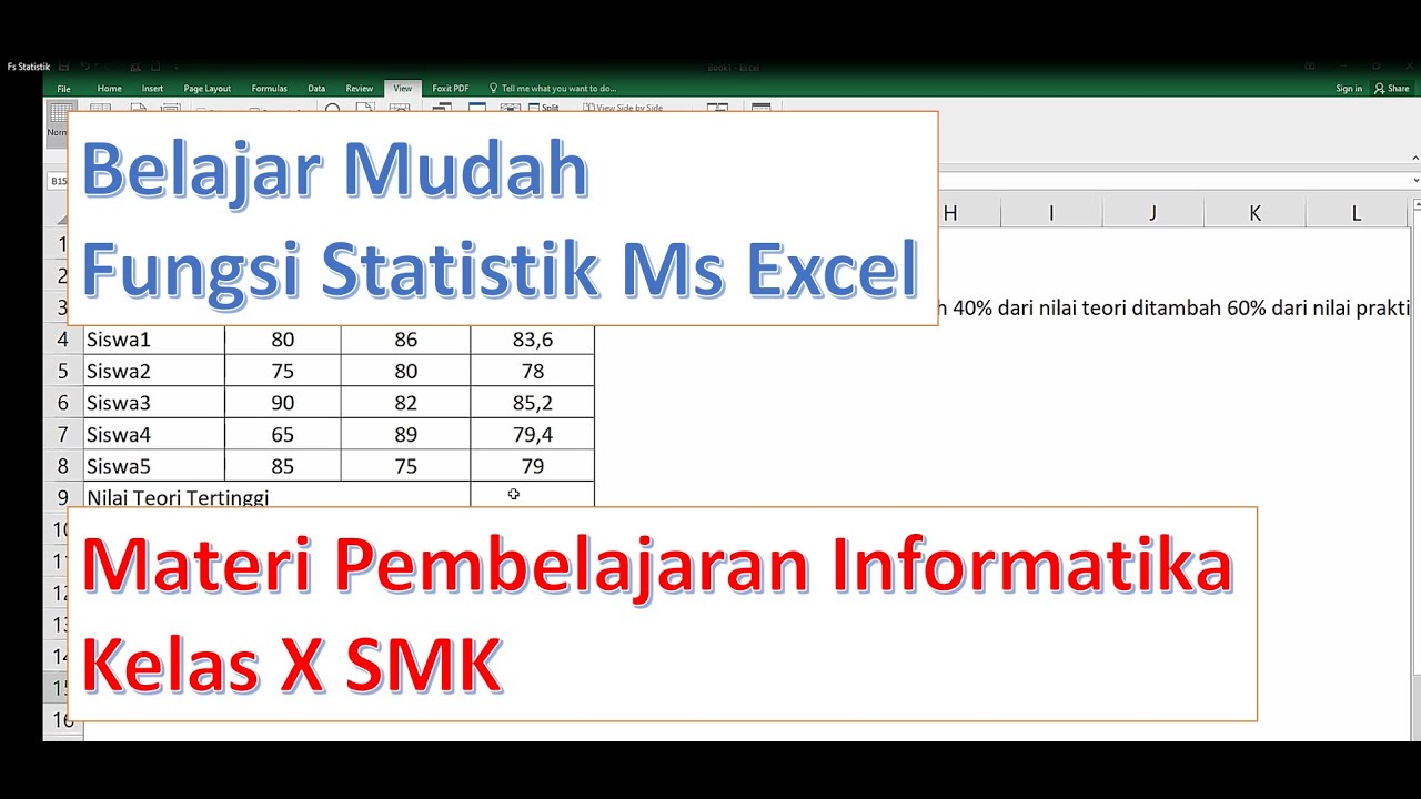
Fungsi Statistik dalam Microsoft Excel - Pembelajaran Informatika Kelas X SMK
Kurikulum Merdeka Informatika Kelas 8 Bab 6 Analisis Data
5.0 / 5 (0 votes)
