What is Digital Signal?

Neso Academy
27 Oct 201508:47

Summary

TLDRThis lecture distinguishes between analog, discrete time, and digital signals. It explains that digital signals discretize both time and magnitude, unlike discrete time signals which only discretize time. The lecture uses temperature and voltage examples to illustrate how digital signals can only take certain fixed levels, leading to quantization errors that can be minimized by increasing the number of levels. The need for digital signals will be discussed in the next lecture.

Takeaways

  • 🕒 The lecture focuses on the concept of digital signals, which are different from analog and discrete time signals.
  • 📊 Digital signals require discretization of both time and magnitude, unlike discrete time signals which only discretize time.
  • ⏱️ Time discretization is achieved by dividing the time axis into equal intervals, calculated using the formula delta T = (Tn - Tn-1).
  • 📉 Magnitude discretization involves dividing the magnitude axis into fixed levels, allowing the signal to take only specific values.
  • 🌡️ An example is given where temperature is measured at discrete time intervals, and then the magnitude is also discretized for a digital signal.
  • 📉 For digital signals, the signal value is rounded down to the nearest allowed level to minimize error, not up, highlighting the importance of selecting the lower value.
  • 🔌 Another example is provided with voltage measurements, where increasing the number of allowed levels reduces the error in signal representation.
  • 📊 Increasing the number of levels in a digital signal allows for more precise measurements and reduces the error compared to fewer levels.
  • 💡 The lecture concludes with a teaser for the next session, which will discuss the necessity of digital signals despite the existence of analog and discrete time signals.
  • 💬 The presenter encourages the audience to think about and share their thoughts on why digital signals are needed in the comments.

Q & A

  • What is the main difference between analog signals and digital signals?

    -Analog signals have continuous values over time, while digital signals are discretized both in time and magnitude, meaning they can only take specific values at specific time intervals.

  • How is the time axis discretized in digital signals?

    -In digital signals, the time axis is discretized by dividing it into equal intervals, which can be calculated using the formula delta T = (Tn - Tn-1) for any given time points Tn and Tn-1.

  • What is meant by discretizing the magnitude axis in digital signals?

    -Discretizing the magnitude axis in digital signals involves dividing the range of possible values into a fixed number of levels, and the signal can only take values that correspond to these levels.

  • Can you provide an example of how temperature is measured in a digital signal?

    -In the example given, the temperature at different times (T1, T2, T3, T4, T5) is measured in degrees Celsius. For a digital signal, the magnitude axis is discretized into levels such as 0, 15, 30, and 45 degrees Celsius, and the temperature at each time point is rounded down to the nearest allowed value.

  • Why is the lower value chosen when a measured value falls between two discrete levels?

    -The lower value is chosen to minimize the error. This approach ensures that the signal value is always closer to the actual measured value than the next higher level would be.

  • How does the number of levels affect the error in digital signals?

    -Increasing the number of levels in a digital signal reduces the error. More levels mean that the discretized values are closer to the actual continuous values, leading to a more accurate representation of the signal.

  • What is the significance of the statement 'the signal can take value equal to this levels only' in the context of digital signals?

    -This statement emphasizes that digital signals are limited to specific, predefined values or levels. They cannot represent values that lie between these levels, which is a key characteristic of digital signals.

  • How is the error reduced when measuring voltage in a digital signal?

    -The error is reduced by increasing the number of levels allowed for the voltage. In the example, when the voltage is discretized into more levels, a voltage of 2 volts can be accurately represented as 2 volts, reducing the error to zero.

  • What is the purpose of dividing the magnitude axis into fixed levels in digital signals?

    -Dividing the magnitude axis into fixed levels allows for easier digital processing and storage of the signal. It also facilitates the transmission of signals with reduced error and complexity.

  • What is the question posed at the end of the script regarding digital signals?

    -The question is: 'If we were already having analog and discrete time signals, then what is the need for digital signals?' This question prompts consideration of the advantages and applications of digital signals over analog and discrete time signals.

Outlines

00:00

📶 Understanding Digital Signals

This paragraph introduces the concept of digital signals, contrasting them with analog and discrete time signals. Digital signals discretize both time and magnitude, whereas discrete time signals only discretize time. The example of measuring temperature at different times (T1 to T5) is used to illustrate the discretization process. In the case of digital signals, the magnitude axis is also discretized into fixed levels (0, 15, 30, 45), and the signal can only take values at these levels. The importance of selecting the lower level to minimize error is emphasized, and the values of temperature at each time point are calculated accordingly.

05:00

🔌 Digital Signal Processing: Reducing Error

This paragraph further explains the difference between digital and discrete time signals using the example of voltage. It demonstrates how digital signals can only take certain values (0 and 5 volts in this case) and how errors can occur when the actual value does not match these levels. The paragraph then explores how increasing the number of levels can reduce this error. By dividing the range into more parts (0, 1.25, 2.5, 3.75, 5 volts), the error can be minimized. The example shows that a voltage of 2 volts is closer to 1.25 volts, so it is assigned that value, reducing the error. The paragraph concludes with a teaser for the next lecture, which will discuss the necessity of digital signals.

Mindmap

Keywords

💡Analog Signal

An analog signal is a continuous signal that can take any value within a certain range. In the context of the video, analog signals are mentioned in contrast to digital signals. The script explains that analog signals can represent temperature or voltage with infinite precision, but they are not the focus of the lecture, which is centered on digital signals.

💡Discrete Time Signal

A discrete time signal is a type of signal where the time axis is sampled at specific intervals, but the magnitude can still take any value within a range. The video script uses the example of measuring the temperature of a city at discrete time intervals (T1, T2, T3, etc.), where the temperature can be any value from 0 to 45 degrees Celsius.

💡Digital Signal

A digital signal is a discrete representation of information where both time and magnitude are quantized into specific levels. The video script emphasizes that digital signals can only take values at predefined levels, such as 0, 15, 30, and 45 degrees Celsius for temperature. This quantization is a key characteristic that distinguishes digital signals from analog and discrete time signals.

💡Discretization

Discretization refers to the process of converting continuous data into discrete data by dividing it into equal intervals or levels. In the video, discretization is applied to both time (delta T) and magnitude (temperature levels). The script uses the example of dividing the magnitude axis into levels to show how digital signals are created from continuous data.

💡Magnitude Axis

The magnitude axis represents the range of possible values that a signal can take, such as temperature or voltage. The video script explains that in digital signals, the magnitude axis is discretized into fixed levels, which is a fundamental concept in digital signal processing.

💡Levels

Levels in the context of the video refer to the quantized values that a digital signal can take. For example, the temperature can only be 0, 15, 30, or 45 degrees Celsius. The script uses the concept of levels to illustrate how digital signals are limited to specific values, which helps in reducing complexity and error in signal processing.

💡Error Minimization

Error minimization is the process of reducing the difference between the original continuous signal and its digital representation. The video script explains that by choosing the lower level when a value falls between two quantized levels, the error can be minimized. This concept is crucial for understanding how digital signals approximate analog signals.

💡Voltage

Voltage is used as an example in the video to illustrate the concept of digital signals. The script discusses how voltage can be discretized into levels of 0 and 5 volts for a digital signal, and how increasing the number of levels can reduce the error in representing the actual voltage.

💡Signal Processing

Signal processing is the analysis and manipulation of signals, which can be analog or digital. The video script focuses on digital signal processing, explaining how signals are discretized and processed in digital systems. Understanding signal processing is essential for grasping the applications of digital signals in various technologies.

💡Quantization

Quantization is the process of approximating a continuous range of values to a discrete set of values. In the video, quantization is applied to the magnitude axis of signals, resulting in digital signals that can only take specific levels. The script uses quantization to explain how digital signals work and how they differ from analog signals.

💡Sampling

Sampling is the process of selecting a subset of data points from a continuous signal at regular intervals. The video script mentions sampling in the context of discrete time signals, where the time axis is sampled, but the magnitude can still vary continuously. Sampling is a fundamental concept in signal processing, especially when transitioning from analog to digital signals.

Highlights

Digital signals require discretization of both time and magnitude axes.

Discretization of time axis involves dividing it into equal intervals.

Magnitude axis discretization involves setting fixed levels for signal values.

In digital signals, the signal can only take values equal to the discretized levels.

Discrete time signals allow any magnitude value within a range.

Digital signals restrict magnitude values to specific levels, like 0, 15, 30, and 45 degrees Celsius.

When a value falls between levels, the lower level is chosen to minimize error.

Increasing the number of levels in digital signals reduces the error.

An example of discretization is given with temperature measurements.

Voltage is another example used to explain digital signal discretization.

Error in digital signals can be reduced by increasing the number of discretization levels.

The difference between discrete time signals and digital signals is highlighted.

The need for digital signals over analog and discrete time signals will be discussed in the next lecture.

The lecture invites viewers to comment their thoughts on the necessity of digital signals.

The lecture concludes with a teaser for the next session's topic.

Transcripts

play00:05

in the last presentation we completed

play00:07

analog and discrete time signal in this

play00:09

lecture we will study digital signal in

play00:11

digital signals we discretize both time

play00:14

and magnitude we have to discretize both

play00:17

time and magnitude axis if you remember

play00:19

the discrete time signals we discretize

play00:21

the time AIS but not magnitude but in

play00:24

case of digital signals we have to

play00:25

discretize the magnitude axis as well by

play00:28

discretization I mean we have have to

play00:30

divide the time XIs in equal intervals

play00:33

if delta T is the interval then we can

play00:36

find out this interval delta

play00:39

T by T1 minus t 0 or we can have T2

play00:44

minus T1 in the same way TN minus TN

play00:50

minus 1 this is how we can find the

play00:52

interval now the next thing that we have

play00:55

to do is to discretize the magnitude

play00:57

axis also this is a very simple example

play01:00

in which we are trying to measure the

play01:02

temperature of a city capital t is the

play01:04

temperature and this is in De Cel small

play01:08

T is the time in seconds and we are

play01:11

measuring the temperature at T1 T2 T3 T4

play01:15

and T5 if I consider the case of

play01:18

discrete time signals then let's see

play01:20

what we have the temperature at time T1

play01:25

is equal to 9° C you can clearly see it

play01:29

is equal to 9° C we have not discretized

play01:32

the magnitude axis so the temperature

play01:35

can take any value from 0 to 45 every

play01:38

value is allowed from 0 to 45 so 9° C is

play01:42

absolutely

play01:43

allowed for

play01:45

T2 for T2 we have

play01:48

38°

play01:50

C for T3 we have 24°

play01:56

C for

play01:58

T4 we have 15 18°

play02:01

C and for T5 we have 45°

play02:06

C and this is for this is for discrete

play02:12

time signal right now we will consider

play02:15

the case of digital signal and we have

play02:17

to discretize this magnitude axis also

play02:19

so let's do it I'm going to discretize

play02:22

this and I will have the next

play02:26

level equal to 15° C and another level

play02:31

equal to 30° C so we have 0 15 30 45 as

play02:36

the allowed values for the temperature

play02:39

capital T this temperature can take

play02:42

values equal to 0 15 3030 and 45 only we

play02:48

divide the magnitude axis into fixed

play02:50

number of levels and the signal can take

play02:53

value equal to this level Sol this line

play02:56

is very important the most important

play02:58

part that you have to remember in

play02:59

digital signals the signal can take

play03:02

value equal to this levels only right

play03:05

now we will consider the same case the

play03:07

same temperatures for the same time and

play03:10

we have to find out what is the value

play03:12

for temperature capital T at these times

play03:16

we are considering the digital signal in

play03:18

this case so let's

play03:20

start temperature T at time

play03:24

T1 at T1 we have 9° C but 9 is not

play03:29

allowed it is between 0 and 15 it is

play03:31

between 0 and 15 now what we have to

play03:35

take 0 or 15 the difference between 0

play03:38

and 9 is 9° C and the difference between

play03:42

9 and 15 is 6° C so this 9° C is near to

play03:48

15° C so at first s it seems we have to

play03:52

consider 15° Celsius but this is not

play03:54

true to minimize the error we have to

play03:57

take the lower value we have to take 0°

play04:01

C this is the key point that you should

play04:03

remember we don't select the higher

play04:05

value we select the lower value so the

play04:07

temperature T at time T1 is equal to 0°

play04:11

C and the temperature T at time T2 is 38

play04:17

but 38 is also not allowed it is between

play04:19

3030 and 45 we again have to take 3030

play04:24

because this is the lower level

play04:27

so at T2 we have we have 30° C

play04:31

temperature T at T3 is equal to at T3 we

play04:36

have 24 24 is near to 30 but again we

play04:39

have to consider the lower level so 15°

play04:43

C is the answer at T4 we have 15 15 is

play04:50

definitely allowed so we have 15° C at

play04:54

T5 we have 45 and 45 is allowed so 45 de

play05:00

C and this is the values in case of

play05:04

digital signal so you can clearly see

play05:07

the difference between discrete time

play05:08

signals and digital signals we can have

play05:11

any value of the temperature within 0 to

play05:14

45 but in this case we have the value

play05:16

for temperature equal to this levels

play05:19

only now we will see one more example in

play05:23

which we will consider the voltage

play05:31

this is the time

play05:33

AIS capital V is the voltage we are

play05:36

considering the digital signal and uh we

play05:39

have 0 volts and 5 volts as the two

play05:44

values that are allowed let's say at any

play05:46

time T1 the

play05:49

voltage is equal

play05:52

to 2 volts then voltage at T1 is equal

play05:58

to 0 volts because I have already

play06:00

explained you we have to consider the

play06:02

lower value so I have taken 0 volts now

play06:05

you can see we have error of 2 volts

play06:10

because the observed voltage was 2 volts

play06:13

but we are getting 0 volts so how to

play06:15

overcome this error we can overcome this

play06:18

error by increasing the number of levels

play06:21

if we

play06:22

increase the number

play06:24

of

play06:26

levels error will reduce this is is very

play06:30

very important Point very very important

play06:33

point on increasing the number of levels

play06:36

arror will reduce let's see how I'm

play06:39

going to divide 0 to 5 in four equal

play06:41

parts so I will

play06:45

have

play06:47

1.25 as the next

play06:50

level

play06:52

2.5 and

play06:55

3.75 okay these are the levels so we now

play06:58

have 0 1.25 2.5 3.75 and 5 as the

play07:04

allowed values for this voltage V so

play07:07

voltage at time T1 is equal to is equal

play07:12

to

play07:13

1.25 volts because we have to consider

play07:17

the lower value and 2 volt is between

play07:20

1.25 and 2.5 now we can easily take 1.25

play07:24

instead of zero so the error is reduced

play07:27

and now we have error error of

play07:31

0.75 volts only earlier the error was 2

play07:35

volts but now the error is

play07:37

0.75 if you increase the number of

play07:40

levels more for example if I have levels

play07:42

equal to 0o 1 2 3 4 and five then this 2

play07:50

volt can clearly be measured as 2 volts

play07:53

so voltage at T1 in this case is equal

play07:57

to 2 volts and

play08:00

error of zero volts is there so we have

play08:05

reduced the error of 2 volts to Zer

play08:08

volts by increasing the number of levels

play08:11

this is all for this presentation but

play08:13

there is one question if we were already

play08:15

having analog and discrete time signals

play08:18

then what is the need of digital

play08:20

signal what

play08:25

is the need of digital

play08:32

signal this is the question and in the

play08:35

next lecture we will discuss this need

play08:37

of digital signal if you know the answer

play08:40

of this question go ahead and post your

play08:42

answer in the comment section this is

play08:44

all for this presentation see you in the

play08:46

next one

Rate This

5.0 / 5 (0 votes)

Etiquetas Relacionadas
Digital SignalDiscretizationSignal ProcessingAnalog vs DigitalMagnitude AxisTime AxisSignal AccuracyError ReductionVoltage LevelsTemperature Measurement
¿Necesitas un resumen en inglés?