Ch 3 Lecture Video, Fall 2024: Measures of Central Tendency

Summary

This educational video script delves into the significance of measures of central tendency in statistical analysis, focusing on mode, median, and mean. It explains how these measures help summarize data, revealing patterns and trends. The script clarifies the concept of range, the calculation of mode as the most frequent value, and the median as the middle value in a dataset. It also discusses calculating the mean, emphasizing its importance in various types of data, including interval, ratio, and ordinal. The script provides examples to illustrate these concepts, aiming to enhance understanding of statistical summaries.

Takeaways

• 📊 Measures of central tendency are crucial for summarizing and analyzing data, helping to understand the 'story' the data is telling.
• 🔢 The concept of 'multivariant' data is introduced, referring to datasets with two or more variables, emphasizing the complexity of modern data analysis.
• 📈 Understanding distributions is key, which involves recognizing how data is spread across different variables and values.
• 🎯 Central tendency focuses on identifying the 'middle point' and typical trends within a dataset, aiding in data summarization.
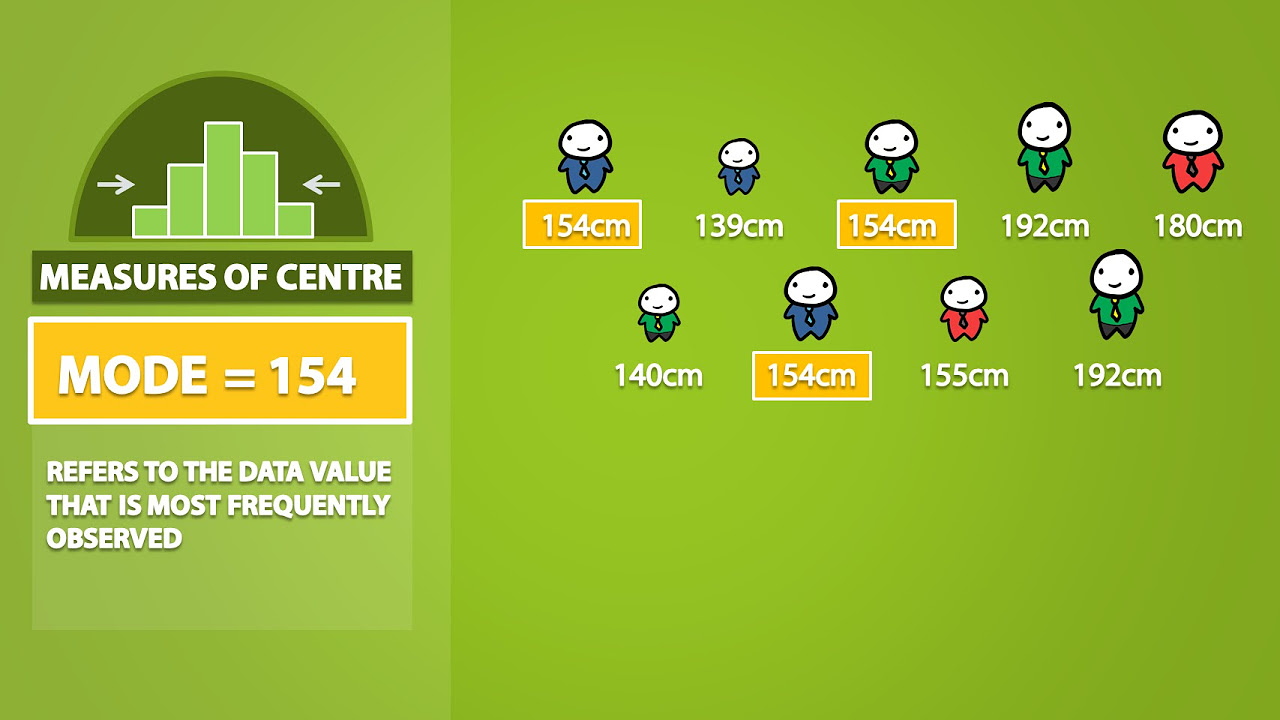
• 🏅 The mode is defined as the most frequently occurring value or category in a dataset, serving as an easy identifier of commonality.
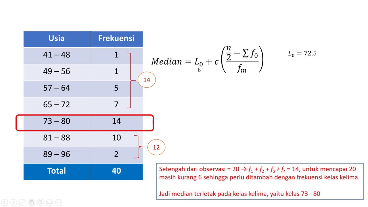
• 🔢 The median is the middle value in a dataset when ordered from least to greatest, dividing the data into halves.
• 📐 The range is calculated as the difference between the highest and lowest values in a dataset, providing a sense of data spread.
• 📊 Percentiles are discussed as a way to understand the relative standing of data points within a dataset, differentiating them from percentages.
• 🧮 The mean, or average, is calculated using the formula \( \bar{Y} = \frac{\sum f \times y}{N} \), where \( f \) is frequency, \( y \) is the value, and \( N \) is the total number of cases.
• ⚖️ Different types of data (nominal, ordinal, interval, ratio) are considered in relation to how they can be analyzed using measures of central tendency, with a clarification that nominal data does not have a mean in the traditional sense.

Q & A

What are the measures of central tendency and why are they important?

The measures of central tendency include mode, median, and mean. They are important because they help summarize data and provide a better understanding of the typical values or patterns within a dataset, allowing for easier analysis and interpretation.

What is the definition of 'distribution' in the context of statistics?

In statistics, 'distribution' refers to how values are spread across categories and variables. It looks at the similarities and differences, essentially showing how data points are dispersed.

Can you explain the concept of 'range' in statistics?

The 'range' in statistics is the difference between the highest and lowest values in a dataset, representing the spread of the data.

What is the mode and how is it determined?

The mode is the value or category that occurs most frequently in a dataset. It is determined by identifying the data point with the highest frequency.

How is the median calculated for a dataset with an odd number of observations?

For a dataset with an odd number of observations, the median is calculated by arranging the data in ascending order and selecting the middle value.

What is the formula used to calculate the mean?

The formula to calculate the mean is the sum of all the values (ΣY) divided by the total number of observations (n), represented as Y Bar = ΣY / n.

How does the calculation of the median differ when the dataset has an even number of observations?

When the dataset has an even number of observations, the median is the average of the two middle values after the data is arranged in ascending order.

What is the significance of assigning numerical values to non-numerical data?

Assigning numerical values to non-numerical data allows for statistical analysis and interpretation, such as calculating means or modes, even when the data is ordinal or nominal.

Why can't nominal data be calculated with a mean in the traditional sense?

Nominal data, which includes categories like gender or eye color, cannot be calculated with a mean in the traditional sense because they do not have a natural order or numerical value that can be averaged.

What is the difference between a percentage and a percentile?

A percentage represents a proportion of a whole, while a percentile indicates the relative standing of a score within a dataset, showing the percentage of cases that fall below a particular value.

Outlines

00:00

📊 Introduction to Measures of Central Tendency

The paragraph introduces the concept of measures of central tendency, emphasizing its importance in statistical analysis. It mentions that understanding variables and frequency distribution tables is foundational, and now the focus shifts to central tendency to better comprehend data. The paragraph highlights the significance of summarizing data to grasp the underlying story it tells. It also touches on the relevance of multivariate data, explaining that it involves dealing with two or more variables. The measures of central tendency discussed include mode, median, and mean, each serving a distinct purpose but collectively aiding in understanding typical value distributions. The text also introduces the term 'distribution' and explains its role in analyzing how values are spread across categories and variables.

05:03

🔢 Exploring the Mode and Median

This paragraph delves into the specifics of the mode and median, two measures of central tendency. The mode is defined as the category or score with the highest frequency, using the example of Spanish being the mode among non-English languages in the United States due to the highest number of speakers. The concept of bimodal distribution is introduced, where two categories have the highest frequencies closely related but not identical. The median is then explained as the middle value of a distribution when data is ordered, with a detailed walkthrough of how to calculate it for both odd and even numbers of data points. The paragraph uses the example of hate crimes reported by states to illustrate the calculation of the median.

10:04

📈 Calculating the Mean and Understanding Percentiles

The paragraph discusses the mean, another measure of central tendency, and provides the formula for its calculation. It explains that the mean represents the average value and is crucial for interval and ratio variables. The text provides an example of calculating the mean for the ideal number of children based on survey responses, demonstrating how to use the formula and interpret the result. Additionally, the concept of percentiles is introduced, explaining how they indicate a score's relative standing within a range, differentiating them from percentages. The paragraph also addresses the calculation of medians in frequency distribution tables and the importance of organizing data to identify the mode.

15:05

📉 Assigning Numerical Values and Grouped Data

This paragraph addresses the process of assigning numerical values to non-numerical data for the calculation of the mean, such as in surveys using Likert scales. It explains how to calculate the mean by multiplying the frequency of each response by its assigned numerical value and then summing these products. The text provides an example involving political views and shows how to interpret the calculated mean in the context of the data. It also touches on the calculation of means for grouped data, such as hours worked, and the assignment of midpoint values to ranges. The paragraph concludes by clarifying that nominal data, which lacks order, does not have a mean calculated in the traditional sense but can be analyzed through percentage breakdowns.

20:06

🚫 Clarification on Nominal Data and Mean Calculation

The final paragraph clarifies that nominal data, such as gender or eye color, does not have a mean calculated in the same way as interval or ordinal data. It emphasizes that while numerical values can be assigned for statistical analysis, these do not represent a central point or average in the same sense. The text provides a clear distinction between calculating percentages, which is similar to means for categorical data, and calculating a mean for ordinal or interval data. It uses the example of calculating the average number of miles driven by individuals to illustrate a straightforward mean calculation. The paragraph reinforces the importance of understanding the nature of data when performing statistical analysis and calculating central tendencies.

Keywords

💡Central Tendency

Central tendency refers to the center point of a data set, which can be represented by measures such as the mean, median, and mode. In the video, central tendency is crucial for summarizing and understanding data distributions. It helps in identifying the typical or average value within a set of data. For instance, the video discusses how measures of central tendency allow for a better understanding of the 'story' the data is telling, highlighting the importance of these measures in statistical analysis.

💡Frequency Distribution Tables

A frequency distribution table is a statistical tool used to organize data into categories and count how often each value or range of values occurs. The video script mentions that understanding these tables is a prerequisite to studying central tendency, suggesting that they are fundamental in building a foundation for statistical analysis. They are used to visualize data and prepare it for further analysis, such as calculating the mode.

💡Mode

The mode is the value that appears most frequently in a data set. It is one of the measures of central tendency discussed in the video. The mode is described as the 'easiest to identify' and is used to determine the most common category or score within a distribution. An example given in the script is the mode for the number of speakers of a language, where Spanish is identified as the mode due to having the highest number of speakers.

💡Median

The median is the middle value in a data set when the numbers are arranged in ascending or descending order. It is another measure of central tendency that the video discusses. The video explains that the median divides the data into two equal halves, with half the values above and half below the median. It is calculated differently for odd and even numbers of data points, as illustrated with examples of hate crimes data and ideal number of children.

💡Mean

The mean, often referred to as the average, is calculated by summing all the values in a data set and then dividing by the number of values. It is a measure of central tendency that the video emphasizes as important for understanding data distributions. The video provides examples of calculating the mean, such as the average number of children people consider ideal or the average number of miles driven by a group of individuals.

💡Range

The range is the difference between the highest and lowest values in a data set, representing the spread of the data. The video introduces the concept of range to understand the dispersion of data values. It is used to identify the extent of variability within a dataset, as shown when calculating the range of points in an example.

💡Multivariate Data

Multivariate data refers to data sets that involve multiple variables. The video script discusses the importance of understanding central tendency in the context of multivariate data, where summarizing and analyzing data with two or more variables becomes necessary. This concept is crucial for handling complex data sets and is part of the progression from univariate to more advanced statistical analysis.

💡Distribution

Distribution in the context of the video refers to the way values are spread across categories and variables. It is a key concept in understanding how data is organized and how it behaves. The video mentions distribution in relation to understanding the spread of values and the similarities and differences within the data, which is essential for identifying central tendencies.

💡Percentiles

Percentiles divide a data set into 100 equal parts and indicate the value below which a certain percentage of observations fall. The video script touches upon percentiles as a way to understand a score's location within a range of data. It explains that a percentile placement, such as the 75th percentile, indicates that 75% of cases are below that score, providing a relative measure of standing within a distribution.

💡Nominal Data

Nominal data refers to categorical data that cannot be ordered, such as gender or eye color. The video clarifies that while nominal data can be organized and counted, it does not have a mean in the statistical sense because it lacks an order or hierarchy. The script uses nominal data as an example to contrast with other types of data, such as ordinal or interval data, where measures of central tendency like the mean can be calculated.

Highlights

Measures of central tendency are crucial for statistical analysis and understanding data.

Understanding variables and frequency distribution tables is fundamental before delving into measures of central tendency.

Measures of central tendency help summarize data and reveal the story it tells.

Multivariate data involves two or more variables and is important for summarizing complex data sets.

Distribution refers to how data is spread across variables and values, showing similarities and differences.

Central tendency focuses on the average or typical patterns or trends within a data set.

Mode is the value or category with the highest frequency in a data set.

Bimodal distribution occurs when two values have the highest frequency.

Median is the middle value in a data set when arranged in order, dividing the data into halves.

Calculating the median involves finding the middle value or averaging the two middle values for even sets.

Mean is calculated by summing all values and dividing by the number of cases.

Mean can be influenced by assigning numerical values to categories in surveys or ratings.

Grouped data requires assigning a midpoint value to each group for mean calculation.

Nominal data, such as gender or eye color, cannot be calculated with a mean but can be presented in percentage breakdowns.

Ordinal data, like stress levels, can have a mean calculated to find a central point.

Understanding measures of central tendency is essential for analyzing and summarizing data effectively.

Transcripts

we're going to talk about the measures

of central tendency because um this is

really one of the the this is really

important part to um moving forward and

getting the work done and starting to

analyze things statistically um you know

we've been doing things in starting to

build our knowledge and understanding

right so far we understand what the

variables are we understand what

frequency distribution tables are we

have an understanding of these things

right so now what we're doing is we're

going to be working with the measures of

central tendency which helps us

understand our data a little bit

more now with this um understanding the

measures of central tendency is

important you know we can use it for our

visuals of course but really it's

important most important because it

allows us to summarize our data it

allows us to summarize our data and be

able to have a better understanding of

what's happening the story it's telling

the P picture that's it's painting right

and so from there um we're able to be

able to work with larger data sets and

more variables uh so the idea of

multivariate data is important because

we might need to summarize more we might

need to summarize things that have more

than just one variable in this case

multivariant means two or more variables

so multi being multiple and then the

variants right being variables so being

able to understand the measures of

central tendency and how that influences

our movement forward um is important

so in terms of the measures of central

tendency um there's a couple there's a

couple words that your book uses and

just kind of acts as if uh you should

understand what they are and one is um

distribution it's used it a lot we're

going to continue using that word and

with distribution it's essentially how

things are distributed right so how it's

spread how it's broken up uh across

variables and values so like it's it's

the similarities and differences so

we're looking at how are spread out how

values are spread out across categories

and

variables for the measures of central

tendency what we're looking at is we're

looking at basically the average or the

typical you know what's average or

typical about the distribution so

thinking about central tendency right

Central where is that kind of Middle

Point and tendency how do what is what

is the what does it tend to do right the

averages or typical um patterns or

trends that are happening with the data

it's essentially looking at categories

and scores and then being able to

describe these things what is typical

across these values so there's three

concepts that we're going to talk about

mode median and mean each of these serve

a different purpose um but they still

highlight typical distributions of

values so they all have a purpose a

different purpose but they still allow

us to see the measures of central

tendency the the distribution of values

within a

category so in chapter 4 on page 100

um it talks about range that's a little

bit of a head a jump ahead but at the

same time um at the same time uh it's

important I think that we talk briefly

about what range is so the range is

basically just that it's the range of

values um what that means is that it's

what is the distance between your lowest

and highest value so if you had like

points for instance 4 6 19 32 79 those

were points your range would be 75

because 79 - 4 right 79 is your highest

value four is your lowest value you'll

also see these little curly brackets and

those are called Curly brackets and they

basically mean discrete values and

that's where you'll see your range the

discrete value is basically um are

values that cannot be subdivided right

so go back to continuous and discreet um

from a couple weeks ago and that's what

we're looking at with our range and the

reason why I bring it range now is

because how can we understand you know

what our our or what the data does what

it tends to do where the center point is

if we don't understand kind of what the

range is our code word is Apple so the

next thing that we're going to talk

about is the mode um the mode is a is

the category or the score with the

largest frequency this does not mean

it's

it's if you had like a rating scale it

does not mean that 10 is your mode

simply because it's the highest number

it's the value or the category that has

the highest number of things that are

occurring it's the easiest to identify

so it's it's essentially the answer or

the selection that somebody chose or

that the most amount of people chose um

you find the category and you find the

highest frequency it's really the

easiest to identify it's the thing that

occurs the most amount of times

um it's the category or the score not

the frequency itself so if it occurred

17 times you're not saying the mode is

17 you're saying the mode is whatever

category or score or value is is there

um if you have something that has more

than you have like two categories that

have the same um are the the highest

though that's called was called bodal so

think about bu being to modal for the

modes um if they're also close but not

exact so like let's say 75 and then 74.8

that is essentially still bodal and you

would report those two highest high you

would still report the two highest

categories or scores um

now the next slide we're going to see

from your book on page it should be on

page 64 uh an example of how mode can

look so in this case they listed as

foreign languages but I'm referring to

it as languages outside of the outside

of languages in the United States out

that are not English and so this is like

the number of speakers on the right and

the language on the left and this is the

number of speakers in those

corresponding

languages in this case Spanish is the

mode now it may not be organized this

way though and it's important that you

understand and identify how you will be

able to organize your data as well

because you're going to have to organize

it it's best to organize it to be able

to see what the mode is in this case

it's easy to identify right we know what

the mode is the mode here then is

Spanish Spanish is the mode because it's

has the highest number of speakers code

word is

pumpkin now the median is different so

the mode is relatively simple because

you can identify it remember it's not

the frequency so in this case it's not

37 million that's not the mode the mode

is Spanish in this case the median is

different because you're going to want

to put things in or in order there is

some sort of logical order not

everything will fit into here but you

can still find the median in the vast

majority of things um but it's the exact

middle of the distribution or the spread

of numbers so in this case it divides it

in half half above and half below um so

you have to sort your data you have to

sort it from you know highest to lowest

or lowest to highest if if it has the

even number of cases you divide it in

half and you do the calculation based

off those if it has an odd number of

cases you use this Formula n+ 1 / 2

where you divide it in half and that is

your is your value and I'm going to show

you on the next couple of slides so it

makes a little more sense so essentially

though the median is where you have your

data and it's half above half below um

and the median is literally that middle

point of the data so in your book this

is the table that it presents to you um

if you look look at it right the number

of hate crimes on the left uh is not in

order it is not in any order it's just

randomly um randomly placed there now if

you look on the right it has the state

and its corresponding state with the

number of hate crimes that occur in it

so we see that there are nine cases

right so we have 1 2 3 4 5 6 7 8 nine so

we have nine cases nine states in this

case then that have reported the number

of hate

crimes now we've reorganized it now

we've ordered it so if you look right

there's no organization now we've

ordered it from fewest to greatest from

least to greatest in terms of amount so

now we can see that this is in some sort

of order still nine cases though now if

you look at this here on the left hand

side this is nine cases so because it's

it's odd we have to use this little

formula so we have nine cases right here

there's nine cases um plus one because

we need to be able to figure out the

middle divided by two so in this case we

get 10 divided two which is five so what

it means is that we need to look at the

fifth case so 1 2 3 4 5 which gives us

Texas right here and that means that 145

is our median that means that that one

Texas here gives us our meeting of 145

so that means half the number of cases

will be fewer than 145 and half the

number of cases will be more than 145 so

that's what the median means is the

middle point now this is for our odd

number of cases but what happens if we

have an even number of cases so we know

that our median is 145 here

let's according to like your textbook

did this so let's say for a minute

California didn't report um we have

eight so we still have this order we've

taken California off so we're pretending

it doesn't exist right now and we have

eight number of cases 1 2 3 4 5 6 7 8

right so what happens is you look at the

two middle so 1 2 3 4 hm 1 2 3 4 H so

that gives us North Carolina and Texas

well what you have to do is you have to

add these two together right here and

divide it by two so gives you your

median and your median is

142.5 so the median basically means that

there are going to be half the amount of

cases that are above 142.5 and half that

are below and this is if you have an

even number of cases you find the two

middle ones you add them together and

divide them into two to get you your

median

number and I'm going to end this video

here and I'm going to create another

video so that way you have them divided

into two

head okay so we're going to go ahead and

um leave off now from where the last

video was and the last video we were

talking about median now you have your

frequency distribution tables and um and

those are useful when we're coming to

when we're trying to figure out our

median right because you've already kind

of organized all the data but what

happens is when you are creating this um

sometimes you have certain categories

that are associated with it so we kind

of already talked about that a little

bit uh and essentially when there's some

sort of category though that isn't

numerical in

value um or is like a different category

in terms of

um what you're trying to measure so on

page 70 it talks about political views

um it says that the the mean uh or not

the mean sorry the the the number um

comes to

21.5 what it's saying is that value is

associated with the label of moderate

and political views and that's what

you're going to go to um so in a couple

slides we'll talk about a little I'll

talk about it a little bit more um in

more detail but that's just something to

think about when it comes to

calculations of um of median for these

categories another thing about this is

um percentiles so you've probably

encountered and experience percentiles a

lot of standardized testing has

percentiles um and with these

percentiles it gives you an idea so a

percentile is not the same as a

percentage it is a general location

within the a range it's a score at or

below a specific range so if you scored

in the 70th 75th percentile it means

that 75% of cases are below it

um and that's a typo so I apologize but

75% of the cases are below it so so that

means that 25% of cases are above that

and it doesn't mean you scored a 75% you

scored could have scored a 20% but you

still are 75 uh in the 75th percentile

or you could have scored 100% but you're

still in the 7 maybe the 75th percentile

because there was extra credit stuff um

so these are things to consider when

we're talking about the calculations of

the medians we'll talk about percentiles

in more detail um at a later point so

now with that um is our mean now and

this calculation this formula here is

super important when I refer to these

things this y here stands for Y Bar this

e is Sigma which means sum the Y so the

combination of these two is the sum of

all your scores your variable scores um

Y Bar means your mean and this n is the

total number of cases and this is the

formula that you use to calculate mean

um there's a couple different ways that

you're going to calculate data values

it's mostly for Interval ratio VAR

variables but it's anything that has a

data value to it and we're going to talk

about this in more you might also hear

it referred to as um average okay so

we're going to talk about that in more

detail um on the next couple of sides to

see how it's applied depending on what

type of data we're using that data

informs um how we move forward with it

so um we're going to go to the next

slide

and oh too far okay so this is um on

page 73 it's in chapter 3 and this is

about the ideal number of children so

essentially this is a survey um

about this is a survey about

um the ideal number of children

and that means that

they were asked what do you believe is

the ideal number of children so the list

here is you know 0 1 2 3 4 5 6 with the

number of

children and frequency is the number of

responses that selected that option so

in this case these were the options zero

children one zero children one child two

children three children four five six

and this is the number of people who

selected these options so 13 people said

zero 16 people said 1 5006 said 2 Etc

which gives us our n at

868 so if you look over at this ex I'm

going to move

this so if you look over at this this

here is Sigma times you or S yeah

Sigma is the sum of your frequency times

your yvalue so your frequency times your

yvalue in this case is frequency times

your y-value the reason you're doing it

this way is because you're trying to

measure the average average number of

children all right that it seems to be

ideal so in this case you have zero you

have 16 you have 1,2 because what you're

doing is you're multiplying your y value

with your frequency so this is 506 * 2

is here so this gives you your n of 868

and then it gives you your your um your

sum of all your y's which is

2139 so what you do if you go back to

that formula is you have

2,100 sorry

2,139 um divided by 868 which comes to

2.46 and so oops so in this case right

that means the ideal number of children

is

2.46 uh we'll talk about how we can

report on this or the different ways

that we can report on this but

ultimately it's totally cool to save

2.46 children um and go and go from

there so what we do is um we're making

this calculation and you're trying to

figure out what what the answer is so in

this case again the ideal number of

children is um

2.46 all

right

now here's a couple things to think

about in terms of calculating mean in a

different in a variety of other ways um

so when we're looking at means this this

one's a little more straightforward in

some ways not this

ah all right so well okay so before this

was a little more straightforward in

terms of the calculations but sometimes

what happens is we have to actually

assign a numerical value to something so

when you're using a linear scale or a

lyer scale um generally these generally

you're you know if or let's say you have

like a value a number value you've

already assigned a numerical value to it

but sometimes you don't and so you'll

just have strongly agree agree neither

disagree Etc and you'll assign a

numerical value to it if you haven't

already now this is then if you have

your frequency this is the number of

times that somebody selected this

option then your frequency same thing

and this is what it comes to the way you

analyze this and you interpret it though

is your mean comes to

2.25 you don't have a 2.25 over here

that doesn't have any value or any

meaning to us right so what happens is

you identify which numerical value

closely aligns to the

2.25 which basically is this neither

agree or disagree so this means that

most people are um you know the average

comes to 2.25 which aligns with neither

agree or disagree so that's essentially

how you're identifying that why you're

how you're using the mean in these types

of linear likey scale

calculations

now there we go um okay so oops okay so

sometimes you're going to have grouped

um things too all right or frequency

ranges and so for you for a lot of you

you use things like hours works or

credits and so similarly like on the

left side hours work 0 1 through 5 6- 10

11 through 15 16 through 20 you assign a

numerical value to that as well because

again you're not calculating this per se

on its own you assign a numerical value

and the reason this is also a good

practice is because if you were to do a

quantitative reasoning class where you

have to do some additional statistical

analysis being able to understand how

you assign a numerical value to it is

important so then you create a frequency

your frequ you include your frequency so

in this case we have this it comes to 32

um and similar to before sorry for

having to move this similar to before

you have the same process right so it's

0 3 10 24

16 and then this comes 2 53 so darn it

um okay so in this

case your mean is 166 now this is kind

of Where It's tricky because it's kind

of arbitrary which means there's no real

rule for it so the way I would say is

like you figure okay well the numerical

value is 1.66 it's kind of divided here

well which really kind of leans more

towards 6.10 but it also means we're not

completely there so really you could say

that most students work within the range

of 1.5 per week but they probably work a

little bit more than that range because

that's essentially what it's telling you

right based off of this mean so that's

how you would calculate some sort of G

grouped frequencies or ranges that you

have

here now um when it so um I realized

that with the nominal data

um I was thinking about it in terms of

your individual questions and I had

worked with most of you and you had like

group frequencies and ranges you had um

a variety of other things and so I

wanted to kind of clarify a things that

I may have said so nominal data itself

can't be calculated with a mean some of

you may actually have Nom and I when I

say nominal data I don't necessarily

mean

um I don't necessarily mean it in terms

of like hours work and such I mean

nominal data specifically in terms of uh

like gender and eye color and even major

uh and so you're not going to have a

mean calculation in the same way you

will have the percent breako breakdown

which is calculated similar to the mean

um but it's not the mean in the typical

way um and the reason I say this is

that you will assign a value to them so

similar to like the previous um slides

and that gives you insight to be able to

run things

statistically but it's not a mean in the

sense that it shows you a point of the

average a use of something or average

water or average hours so if I said that

you would have a mean for everything the

vast majority of things will have a mean

some things will only have a mode if

it's only a category um so sometimes

your data you know if it's ordinal data

you will have it and for a lot of your

projects most of you have like interval

Ratio or ordinal um but thinking about

some of the major ones like major that

is nominal and that's not going it

doesn't have any order so you can

calculate these averages right um but

they don't have a statistical meaning in

the same way and so I just wanted to

make sure I clear that up if there was

any confusion about what I was saying um

which is why for some of you when I said

to have these uh I perhaps the better

way I should have said is like have it

set up to where you will have two rows

two columns um and you can calculate

those things in terms of that break so

some of your frequency distribution

tables will be enough for that but

essentially in this case you're um you

you can calculate percentages which is

essentially very similar um and that was

my confusion um based off of the number

of projects that I've been working on

closely with all of you um so I just

wanted to kind of clear that up um but

it is important when we're talking about

some of the two column ones that I was

asking you to do uh which will arise um

in terms of your projects so for

instance you're thinking let's say you

want to know you have been talking to

these five people Sam Charlie Sarah Max

and Joe and you want to know what the

average or mean number of miles driven

in a year between these people are so

you asked you ask them how many miles

have you driven in this past year and

they give you this variety of things so

Sam gives you

7,335 Charlie's

36295 Sarah is

21523 Max is 10,23 5 and Jo's 12

567 so in order to come up with your

mean it's going to be very similar to

where you calculate all of those numbers

um and you divide it by the number of

cases so in this case you add these all

up comes to 87,000 955 you divide it by

the total number of people which is five

um which means that your mean miles

driven is 17591 and that's it that's all

you have to do for this uh mean um or

average calculation so really the big

thing is to think about like because

there's no order to eye color there's no

order to um any of those things but if

you had like a category that was ordinal

in terms of like stress levels or

um a variety of those things then that's

where you would calculate the mean you

will calculate percentages which are

still kind of like averages in a way but

you're not assigning some sort of

hierarchal value or statistical value to

it in the sense that it will inform or

influence some sort of Central Point and

so that was that's kind of what I wanted

to clear up and clarify here um so

that's all there is for measures of

central tendency so you are going to be

thinking about these things as you move

forward