03. Cómo describir una variable numérica | Curso de SPSS

BIOESTADISTICO

18 Aug 201506:52

Summary

TLDRThis script discusses key statistical measures for summarizing numerical data. It covers measures of central tendency (mean, median, mode), dispersion (standard deviation, variance, and standard error), position (percentiles, quartiles, deciles), and shape (skewness, kurtosis). The script uses examples like age, weight, and height to explain these concepts, highlighting how they help understand data distribution and variability.

Takeaways

📊 Describing a numerical variable involves summarizing it through various measures: central tendency, dispersion, position, and shape.
🔢 Central tendency measures include the mean (average), median (middle value), and mode (most frequent value). A normal distribution has the same mean, median, and mode.
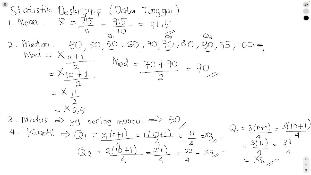
🧮 Mean is calculated by summing all data points and dividing by their count. Median is the middle value when data is ordered. Mode is the most repeated value.
📉 Dispersion measures like standard deviation, variance, and standard error indicate how spread out the data is relative to the mean.
📏 Standard deviation shows data spread relative to the mean, variance is the square of standard deviation, and standard error is the standard deviation of the mean.
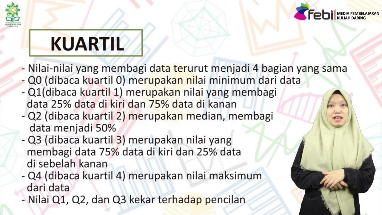
📋 Position measures such as percentiles, quartiles, and deciles divide data into 100, 4, and 10 equal parts, respectively, to understand data distribution.
📊 Quartiles (Q1, Q2, Q3) and percentiles (e.g., P23) are specific types of position measures that provide insights into data distribution.
📈 Shape measures like skewness and kurtosis are quantified by the skewness coefficient and kurtosis coefficient, indicating the symmetry and peakedness of the data distribution.
🔄 Positive skewness indicates a right tail, negative skewness indicates a left tail, and zero skewness suggests a symmetrical distribution.
📊 Kurtosis measures the 'tailedness' of the distribution; positive kurtosis indicates a leptokurtic distribution, negative indicates a platykurtic distribution, and zero suggests a mesokurtic distribution.

Q & A

What are the main types of measures used to summarize numerical variables?
-The main types of measures used to summarize numerical variables are measures of central tendency, measures of dispersion, measures of position, and measures of shape.
What are the three most common measures of central tendency?
-The three most common measures of central tendency are the mean (average), median, and mode.
How is the mean calculated and what is an example from the script?
-The mean is calculated by summing all the data points and dividing by the number of data points. An example from the script is the mean age of a group of people, which is 31 years.
What is the median and how does it relate to the data set's order?
-The median is the value that lies in the middle of a data set when it is ordered from least to greatest. In the script, the median age is 29 years.
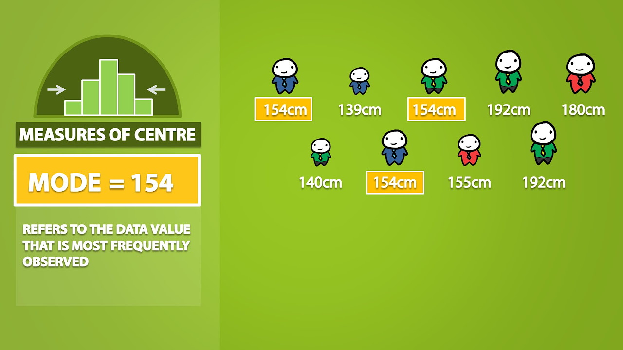
What is the mode and what does it indicate about the data?
-The mode is the value that appears most frequently in a data set. It indicates the most common value among the data points. In the script, the mode of age is 27 years.
If the mean, median, and mode of a distribution are the same, what does this suggest about the distribution?
-If the mean, median, and mode are the same, it suggests that the distribution is normal.
What are the primary measures of dispersion and how do they differ?
-The primary measures of dispersion are the standard deviation, variance, and the standard error. The standard deviation measures how spread out the data is from the mean. Variance is the square of the standard deviation and is used in most statistical procedures. The standard error is a measure of how spread out the sample means are from the population mean.
What is the standard error of the mean and why is it important?
-The standard error of the mean is a measure of how much variability or 'spread' exists in the sample means over all possible samples. It is important because it provides an estimate of how close the sample mean is likely to be to the true population mean.
What are measures of position and how are they calculated?
-Measures of position include percentiles, quartiles, and deciles. They are calculated by dividing the data set into 100, 4, and 10 equal parts respectively, and identifying the values that correspond to these divisions.
What is the significance of the 23rd percentile mentioned in the script?
-The 23rd percentile mentioned in the script is an example of a measure of position that divides the data set into 100 parts and identifies the value that corresponds to the 23rd part.
What are measures of shape and how are they used to describe a distribution?
-Measures of shape include skewness and kurtosis. They are used to describe the shape of a distribution's tails. Skewness measures the asymmetry of the distribution, while kurtosis measures whether the distribution is peaked or flat relative to a normal distribution.
What does a positive skewness coefficient indicate about a distribution?
-A positive skewness coefficient indicates that the distribution has a longer tail on the right side, meaning there are more values on the higher end of the distribution.
What does a positive kurtosis value suggest about the distribution?
-A positive kurtosis value suggests that the distribution is leptokurtic, meaning it is more concentrated around the mean and has heavier tails compared to a normal distribution.

Outlines

00:00

📊 Descriptive Statistics Overview

This paragraph introduces the concept of descriptive statistics for numerical variables. It explains that numerical variables can be summarized using measures of central tendency, dispersion, position, and shape. The paragraph then delves into the specifics of each category, starting with measures of central tendency such as the mean (average), median (middle value), and mode (most frequent value). It provides an example using the variable 'age', where the mean age is 31 years, the median is 29 years, and the mode is 27 years. The paragraph also discusses measures of dispersion, including standard deviation, variance, and standard error, using 'weight' as an example. It mentions that standard deviation and variance are used to understand how spread out the data is from the mean, with standard deviation being in the same units as the original variable and standard error being an estimate of the variability of the mean.

05:00

📈 Position and Shape Measures in Statistics

The second paragraph continues the discussion on descriptive statistics by focusing on measures of position and shape. It explains the concept of percentiles, quartiles, and deciles as measures of position, which divide a dataset into equal parts to identify specific values at certain points. The paragraph gives an example using the variable 'height', where quartiles (Q1, Q2, Q3) and the 23rd percentile are calculated. Measures of shape, such as skewness and kurtosis, are also introduced. Skewness is measured by the coefficient of asymmetry, which indicates whether the data distribution is skewed to the right (positive) or left (negative). Kurtosis is measured by the coefficient of peakedness, which describes the shape of the distribution's tails. The paragraph concludes with an example using the variable 'body mass index', where the coefficient of asymmetry is positive (right skew) and the kurtosis is also positive, indicating a leptokurtic distribution.

Mindmap

Keywords

💡Central Tendency Measures

Central tendency measures are statistical values that describe the center point of a dataset. In the video, three central tendency measures are discussed: mean, median, and mode. The mean is the average value obtained by summing all data points and dividing by the number of data points. The median is the middle value when the data is ordered, and the mode is the value that appears most frequently. These measures are crucial for summarizing and understanding the general trend within a dataset. For instance, the video mentions calculating the mean, median, and mode for a variable 'age', resulting in values of 31 years, 29 years, and 27 years respectively.

💡Dispersion Measures

Dispersion measures are used to quantify the amount of variation or dispersion within a dataset. The video script mentions three key dispersion measures: standard deviation, variance, and standard error. The standard deviation indicates how spread out the data is relative to the mean, variance is the square of the standard deviation, and the standard error is a measure of how much the sample mean is expected to vary from the true population mean. These measures are essential for understanding the variability within a dataset, as illustrated by the calculation of the standard error and variance for the 'weight' variable in the video.

💡Position Measures

Position measures, such as percentiles, quartiles, and deciles, divide a dataset into equal parts and help to understand the relative standing of data points within the dataset. Quartiles divide the data into four equal parts, with each part representing 25% of the data. Percentiles divide the data into 100 equal parts, and deciles divide it into 10 equal parts. The video provides an example of calculating quartiles (25th, 50th, and 75th percentiles) and a specific decile (23rd percentile) for a 'height' variable.

💡Shape Measures

Shape measures describe the shape of the distribution of a dataset. The video discusses two shape measures: skewness and kurtosis. Skewness measures the asymmetry of the distribution, with positive skew indicating a tail on the right (asymmetrical to the right) and negative skew indicating a tail on the left. Kurtosis measures the 'tailedness' of the distribution, with positive kurtosis indicating a more pointed peak and negative kurtosis indicating a flatter peak. The video gives an example of calculating skewness and kurtosis for the 'body mass index' variable, indicating a right-skewed and leptokurtic distribution.

💡Mean

The mean, also known as the arithmetic mean, is a measure of central tendency that represents the average value in a dataset. It is calculated by adding all the values together and then dividing by the number of values. In the video, the mean is used to describe the average age of a group of people, which is given as 31 years.

💡Median

The median is another measure of central tendency that represents the middle value of a dataset when the values are arranged in ascending order. If there is an even number of observations, the median is the average of the two middle numbers. The video script uses the median to describe the central value of the 'age' variable, which is 29 years.

💡Mode

The mode is the value that occurs most frequently in a dataset. It is the only central tendency measure that is not necessarily a numeric value and can be used with both numerical and categorical data. In the video, the mode is used to describe the most common age in the dataset, which is 27 years.

💡Standard Deviation

Standard deviation is a dispersion measure that quantifies the amount of variation or dispersion in a set of values. It is calculated as the square root of the variance and represents the average distance of each data point from the mean. The video mentions calculating the standard deviation for the 'weight' variable, which is 9.33 in the original units of kilograms.

💡Variance

Variance is the average of the squared differences from the mean. It is a measure of dispersion that indicates how far a set of numbers is spread out from their average value. The video script refers to variance as the square of the standard deviation and uses it to describe the variability of the 'weight' variable.

💡Standard Error

Standard error is a measure of how much the sample mean is expected to vary from the true population mean. It is calculated as the standard deviation divided by the square root of the sample size. The video script uses the standard error to describe the variability of the sample mean for the 'weight' variable, which is 1.2.

💡Quartiles

Quartiles divide the data into four equal parts, with each part representing 25% of the data. Q1 represents the 25th percentile, Q2 is the median or 50th percentile, and Q3 is the 75th percentile. The video script provides an example of calculating quartiles for the 'height' variable, which helps to understand the distribution of heights within the dataset.

Highlights

Numeric variables can be summarized using measures of central tendency, dispersion, position, and shape.

Central tendency measures include the mean, median, and mode.

The mean is calculated by summing all data points and dividing by the number of data points.

The median is the middle value when all data points are ordered.

The mode is the value that appears most frequently in the data set.

A normal distribution has the same mean, median, and mode.

Dispersion measures include standard deviation, variance, and standard error.

Standard deviation indicates how spread out the data is relative to the mean.

Variance is the square of standard deviation and is used in most statistical procedures.

Standard error is a measure of how spread out the sample mean is from the population mean.

Position measures include percentiles, quartiles, and deciles.

Percentiles divide the data into 100 parts, quartiles into four, and deciles into ten.

Shape measures include skewness and kurtosis, which are measured by skewness and kurtosis coefficients.

Skewness is positive for right-skewed data and negative for left-skewed data.

Kurtosis is positive for leptokurtic distributions, negative for platykurtic distributions, and zero for mesokurtic distributions.

The transcript provides a detailed analysis of descriptive statistics for variables such as age, weight, height, and body mass index.

The mean age of the group is 31 years, with a median of 29 years and a mode of 27 years.

The standard error for weight is 1.2, and the standard deviation is 9.33 kilograms.

Quartiles for height are the 25th, 50th, and 75th percentiles.

The body mass index has a positive skewness coefficient, indicating right-skewed data.

The body mass index also has a positive kurtosis coefficient, indicating a leptokurtic distribution.