REGRESSION AND CORRELATION EDDIE SEVA SEE

Summary

This educational video script delves into the concepts of regression and correlation using Excel. It explains regression as a statistical method for estimating dependent variable values based on independent variables, utilizing the least squares method to determine the regression line's slope and y-intercept. The script provides a step-by-step guide on implementing simple linear regression in Excel, including calculating predicted values. It also explores correlation, specifically Pearson's R, to measure the strength and direction of the relationship between two variables. The script concludes with a discussion on the implications of these statistical measures for research and decision-making.

Takeaways

• 📊 **Regression Analysis**: Regression is a statistical method used to estimate the value of a dependent variable based on the value of an independent variable, minimizing the sum of squared differences.
• 🔍 **Minimizing Errors**: The regression line is determined by minimizing the squared sum of the differences between the actual and estimated values of the dependent variable.
• ✏️ **Partial Derivatives**: Partial derivatives are applied to find the slope (B) and y-intercept (a) of the regression line, which are crucial for the linear regression equation.
• 📈 **Slope and Y-Intercept**: The slope indicates how much the dependent variable changes with each unit change in the independent variable, while the y-intercept is the value of the dependent variable when the independent variable is zero.
• 📝 **Excel Implementation**: Excel can be used to perform linear regression by programming formulas for B, A, and Y_current, allowing for predictions based on historical data.
• 🔮 **Forward and Backward Estimation**: Regression allows for both forward estimation (predicting future values) and backward estimation (estimating past values) based on the regression formula.
• 🔗 **Correlation**: Correlation measures the statistical relationship between an independent and a dependent variable, with Pearson R being a common measure to determine the strength and direction of this relationship.
• 📉 **Negative Correlation**: A negative correlation indicates that as the independent variable increases, the dependent variable decreases, and vice versa.
• 📊 **Excel for Correlation**: Excel can calculate Pearson R quickly using its statistical functions, providing insights into the relationship between two variables.
• 🔎 **Inferential Statistics**: In research, inferential statistics is important for generalizing findings from a sample to a larger population, often involving significance tests to validate relationships.

Q & A

What is the definition of regression as discussed in the script?

Regression is a statistical process of estimating the value of the dependent variable, given the value of the independent variable, using the regression line determined by minimizing the square of the sum of the differences between the true or historical value of the dependent variable and the estimated value.

How does the slope of the regression line (B) provide information about the dependent variable?

The slope of the regression line (B) indicates how much the value of the dependent variable changes for every unit change of the value of the explanatory variable.

What is the significance of the y-intercept (a) in a regression model?

The y-intercept (a) gives the value of the dependent variable when the value of the explanatory variable is zero.

What method is used to determine the formulas for the slope (B) and y-intercept (a) in a regression model?

The formulas for the slope (B) and y-intercept (a) are determined by applying partial derivatives to the equation of the sum squared errors and solving for the minimum.

How can Excel be used to perform linear regression?

Excel can be used to perform linear regression by programming the formulas for B, A, and Y current in the respective cells and using the historical data to solve for the values of A and B.

What is the simple linear regression formula used in Excel as mentioned in the script?

The simple linear regression formula used in Excel is Y current equals a plus B times X.

Can you explain the concept of correlation as discussed in the script?

Correlation is a statistical relationship between an independent or explanatory variable and a dependent variable. It measures the extent to which the same individual occupies the same relative position on two variables.

What is the role of Pearson R in determining the correlation between two variables?

Pearson R is used to determine the measure of correlation between two variables. It represents how closely the trend between two sets of data from the explanatory and dependent variables aligns.

How can Excel be used to compute the Pearson correlation coefficient?

Excel can compute the Pearson correlation coefficient by using the 'Pearson' function under the statistical category in the formulas menu, where you input the ranges for the two variables.

What does a negative Pearson correlation coefficient indicate about the relationship between two variables?

A negative Pearson correlation coefficient indicates that as the value of the independent variable increases, the value of the dependent variable decreases, and vice versa.

How can the magnitude of the Pearson correlation coefficient be interpreted in terms of the relationship between variables?

The magnitude of the Pearson correlation coefficient indicates the strength and direction of the linear relationship between two variables. A coefficient close to -1 or 1 indicates a strong relationship, while a coefficient close to 0 indicates a weak relationship.

Outlines

00:00

📊 Introduction to Regression and Correlation in Excel

This paragraph introduces the concepts of regression and correlation using Excel. Regression is explained as a statistical method for estimating the value of a dependent variable based on the value of an independent variable, using the regression line. The process involves minimizing the sum of squared differences between the actual and estimated values of the dependent variable. The paragraph details how to calculate the slope (B) and y-intercept (a) of the regression line using partial derivatives. It also provides a practical example of predicting sugar sales for week 12 based on historical data from weeks one to ten. The process of inputting formulas in Excel to calculate the regression coefficients and predict future values is described, culminating in an example where the predicted sales for week 12 are shown as 30.2242 units.

05:01

🔗 Exploring Correlation and its Significance

The second paragraph delves into the concept of correlation, specifically using Pearson's R to measure the statistical relationship between an independent and a dependent variable. It emphasizes that while correlation can indicate the strength and direction of a relationship, it does not prove causation. An example is provided where the relationship between the price and demand for sugar over ten weeks is analyzed. The paragraph explains how to use Excel's statistical functions to compute Pearson's R, and it discusses the interpretation of a negative correlation coefficient, indicating an inverse relationship between the price of sugar and its demand. The significance of this relationship is highlighted, showing how a strong negative correlation suggests that an increase in price leads to a decrease in demand, and vice versa.

10:01

📉 The Implications of Correlation in Research

The final paragraph discusses the implications of correlation measurements in research, particularly the difference between findings from probability and non-probability samples. It points out that while non-probability samples limit conclusions to the sample itself, probability samples allow for broader inferences about the population. The paragraph underscores the importance of inferential statistics in research, suggesting that correlation measures can indicate trends that are likely to be true in the broader population. It concludes by summarizing the discussion on regression and correlation, thanking the audience for their engagement.

Keywords

💡Regression

Regression in the context of the video refers to a statistical method used to estimate the relationship between variables. It involves using a line (regression line) to predict the value of a dependent variable based on the value of an independent variable. The process minimizes the sum of the squared differences between observed and predicted values. In the video, regression is used to estimate sales of sugar at week 12 using historical data from weeks one to ten.

💡Correlation

Correlation is a measure of the strength and direction of the relationship between two variables. The video discusses Pearson's R, a specific type of correlation coefficient that quantifies the linear relationship between two sets of data. A high negative correlation, as illustrated with the example of sugar prices and demand, suggests that as one variable increases, the other decreases.

💡Dependent Variable

The dependent variable is the variable that is being predicted or explained by the independent variable in a regression analysis. In the video, the sales of sugar are the dependent variable, with the aim to predict its value based on the independent variable, which in this case is the week number.

💡Independent Variable

The independent variable is the variable that is used to predict the value of the dependent variable. In the video, the week number is the independent variable, with the assumption that it influences the sales of sugar, the dependent variable.

💡Linear Regression

Linear regression is a specific type of regression analysis where the relationship between the independent variable and the dependent variable is modeled using a straight line. The video uses linear regression to predict sugar sales based on the week number, with the formula Y = a + BX, where Y is the dependent variable, X is the independent variable, a is the y-intercept, and B is the slope.

💡Slope

The slope (B) in a linear regression model represents the amount of change in the dependent variable for a one-unit change in the independent variable. The video explains how the slope can be calculated using partial derivatives and is crucial for understanding how the sales of sugar change with each passing week.

💡Y-Intercept

The y-intercept (a) in a linear regression model is the point where the regression line crosses the y-axis. It represents the expected value of the dependent variable when the independent variable is zero. In the video, the y-intercept is part of the formula used to predict sugar sales when the week number is zero.

💡Partial Derivatives

Partial derivatives are used in the video to minimize the sum of squared errors in a regression model. They are a mathematical technique for finding the slope and y-intercept of the regression line by differentiating the equation with respect to the parameters a and B.

💡Pearson R

Pearson R, mentioned in the video, is a measure of correlation that reflects the strength and direction of a linear relationship between two variables. A negative Pearson R value, as discussed in the context of sugar prices and demand, indicates a strong inverse relationship, where an increase in one variable corresponds to a decrease in the other.

💡Excel

Excel is a software application used for spreadsheets, data analysis, and visualization. The video demonstrates how to use Excel for performing regression and correlation analysis. It shows how to input data, program formulas for calculating regression coefficients, and use Excel's built-in functions to compute Pearson's R.

Highlights

Regression is a statistical process for estimating the value of a dependent variable based on the value of an independent variable.

The regression line is determined by minimizing the sum of the squared differences between the actual and estimated values.

Partial derivatives are used to find the slope and y-intercept of the regression line.

The slope of the line indicates the change in the dependent variable for each unit change in the explanatory variable.

The y-intercept represents the value of the dependent variable when the explanatory variable is zero.

The simple linear regression formula is Y_current = a + BX, where a and B are constants derived from the data.

Historical data is necessary to solve for the values of a and B in the regression formula.

Excel can be used to program and solve for the values of a and B in a regression model.

An example is provided to illustrate how to estimate future sales of sugar using regression.

Correlation measures the statistical relationship between an independent and a dependent variable.

Pearson R is a measure of correlation that indicates the extent to which two variables move in relation to each other.

A negative correlation suggests that as one variable increases, the other decreases, and vice versa.

Excel can be used to compute the Pearson R value for a set of data to determine the strength and direction of the correlation.

A strong negative correlation between price and demand for sugar suggests that higher prices lead to lower demand.

Correlation measures do not prove causation, but they can indicate a relationship between variables.

The significance of the correlation can be tested to determine if the trend is likely to hold in the population.

Inferential statistics is crucial for extending findings from a sample to a broader population.

The lecture concludes with a summary of the discussed topics: regression and correlation.

Transcripts

hello students and fellow researchers

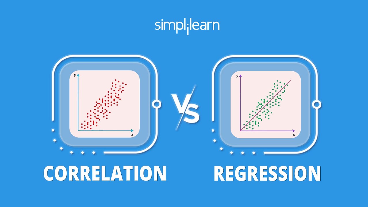
I am going to discuss

regression and correlation using Excel

regression is a statistical process of

estimating the value of the dependent

variable forward or backward

given the value of that independent

variable

using the regression line

determined by minimizing the square of

the sum of the difference between the

true or historical value of the

dependent variable

and estimated value of the same

using partial derivatives

and determining the formulas or

solutions for the slope of the line and

the y-intercept

the slope of the line provides

information on how much the value of the

dependent variable changes

for every unit change of the value of

the explanatory variable

the y-intercept gives the value of the

dependent variable when the value of the

explanatory variable is zero

applying partial derivatives with

respect to a and with respect to B to

the equation of the sum

squared errors results to the following

equations which are actually the

equations for a and b

the values of A and B using the

corresponding formulas can be

substituted to the equation Y current

equals a plus BS

as shown

the minimization process yields the

formula for the slope of the line B and

the y-intercept a

values which can be solved when the

historical data of the variables are

collected or observed

when b and a are determined they serve

as the constant a and the coefficient B

of the simple linear regression formula

why current equals a plus BX

let us now consider as an illustration

for the simple linear regression this

case

for the consecutive's weeks one to ten

the sales in units for sugar each week

are shown in the data set shown in the

next template

what would be the sales for sugar at

week 12.

this is

the

Excel sheet showing the collected or

historical data

for which

X and sales y

in other words

what is y current when X is 12.

to be able to use the linear regression

why Clarity equals a plus BX we must

solve for the values of A and B

we need to program in Excel the formulas

for B A and Y current

this is the Excel sheet that shows the

programming

encode the following programs in the

respective cells So the instructions are

given in the space

and of course the Excel sheet

is also shown where the programs are

inputted

in continuation this page also shows the

other

programs

another page for the continuation of the

programs

and actually

finally

in j6

the answer is given that is 30.2242

regression enabled us to estimate

forward the value of the dependent

variable at least 12.

in as much as the solution has been

programmed

or any new higher value of x the Excel

sheet will automatically predict the

value of y if you make use of any

earlier value of x a backward estimate

of the value i y will also be performed

by the formula

the forward or backward estimate of the

value of y is our process of regression

we proceed to the next topic correlation

correlation is a statistical

relationship between an independent or

explanatory variable and a dependent

variable

Pearson R is used

to

determine the measure of correlation

personal sample R represents the extent

to which the same individual

respondent object or subject

occupies the same relative position on

two variables

it shows how close the trend between two

sets of data from the explanatory and

dependent variables is

if the data are not from an experiment

the relationship will not prove

causation

this is our illustrative example

for the consecutive weeks one to ten the

demand and units and price per unit for

sugar each week

a shown in the data set in the next

template

what is the magnitude of relationship

between price of and demand for sugar

this is the formula for Pearson r

however we can use the program in Excel

for faster computation

this is the Excelsior showing the data

the price

versus the demand

for sure

to use the Excel program

click formulas

click more functions

click the statistical

click Pearson

the carry effects appears

type A2 colon a11 in array1

type B do colon b11 and array2

what does negative

0.98896 mean

the negative sign means that as the

value of the independent or explanatory

variable increases

the value of the dependent variable

decreases or

as the former decreases the latter

increases

the value negative

0.98896 further means

for every 100 percent increase in the

value of the independent variable

there is a

98.896 percent decrease in the value of

the dependent variable

or for every 100 percent decrease in the

value of the former

there is a

98.896 percent increase in the value of

the latter

this also means that

98.896 percent of the change in the

value of the dependent variable

can be accounted for or explained by the

100 change in the value of the team

dependent variable

measures of relationship or Association

present

the closeness of or the similarity in

the trend of the change in values of one

variable with respect to the change in

values of another variable

it shows the parallelism in the changes

in the two variables as in our previous

example between price of sugar and

demand for sugar

the very strong negative relationship

between the two could lead you to

hypothesize that as the price of sugar

grows higher

than in the demand for the product

lowers

if you computed a very very low

Association

for instance between number of trainings

and performance this could be a basis of

your premise

that the quantity of trainings would

have no bearing on your employees

performance

well the measure of Association

indicates the trend in the changes of

values

present in the samples of serving

they do not directly point to the trend

of values

in the entire population

in probability samples these measures of

relationship could actually show if the

trend is more likely true also in the

population represented

by testing the significance of the

relationship

in research undertakings

inferential statistics is very important

a non-probability example that does not

have a scientifically accepted support

for inferential analysis

commonly termed as significance tests

would have to limit the findings

conclusions and recommendations to the

research sample

from a probability sample however

the findings conclusions and

recommendations could be applied to the

concerned population of the study

today we have discussed regression and

correlation

thank you for listening reading

and viewing