The Empirical Rule

Summary

The video script explains the Empirical Rule, which is used for visualizing data with a bell-shaped distribution. It highlights that approximately 68% of data falls within one standard deviation, 95% within two, and 99.7% within three standard deviations from the mean. The rule is significant as it allows for the estimation of the bell curve's shape using just the mean and standard deviation. The script also demonstrates how to apply the Empirical Rule to a dataset with a mean of 50 and a standard deviation of 10, showing that the rule can accurately predict data distribution, provided the data is normally distributed.

Takeaways

• 📊 The Empirical Rule is a method to visualize data distribution when it is assumed to be bell-shaped or normally distributed.
• 🔢 According to the Empirical Rule, 68% of data points fall within one standard deviation of the mean.
• 📉 About 95% of data points are within two standard deviations of the mean in a normal distribution.
• 📈 Almost all (99.7%) data points (with a few exceptions) are within three standard deviations of the mean.
• 📋 For a dataset with a mean of 50 and a standard deviation of 10, 68% of observations would be between 40 and 60.
• 📐 The Empirical Rule helps to estimate the shape of the bell curve using only the mean and standard deviation.
• 📈 When drawing the bell curve, the tails are drawn with different slopes to represent the data distribution outside of one, two, and three standard deviations.
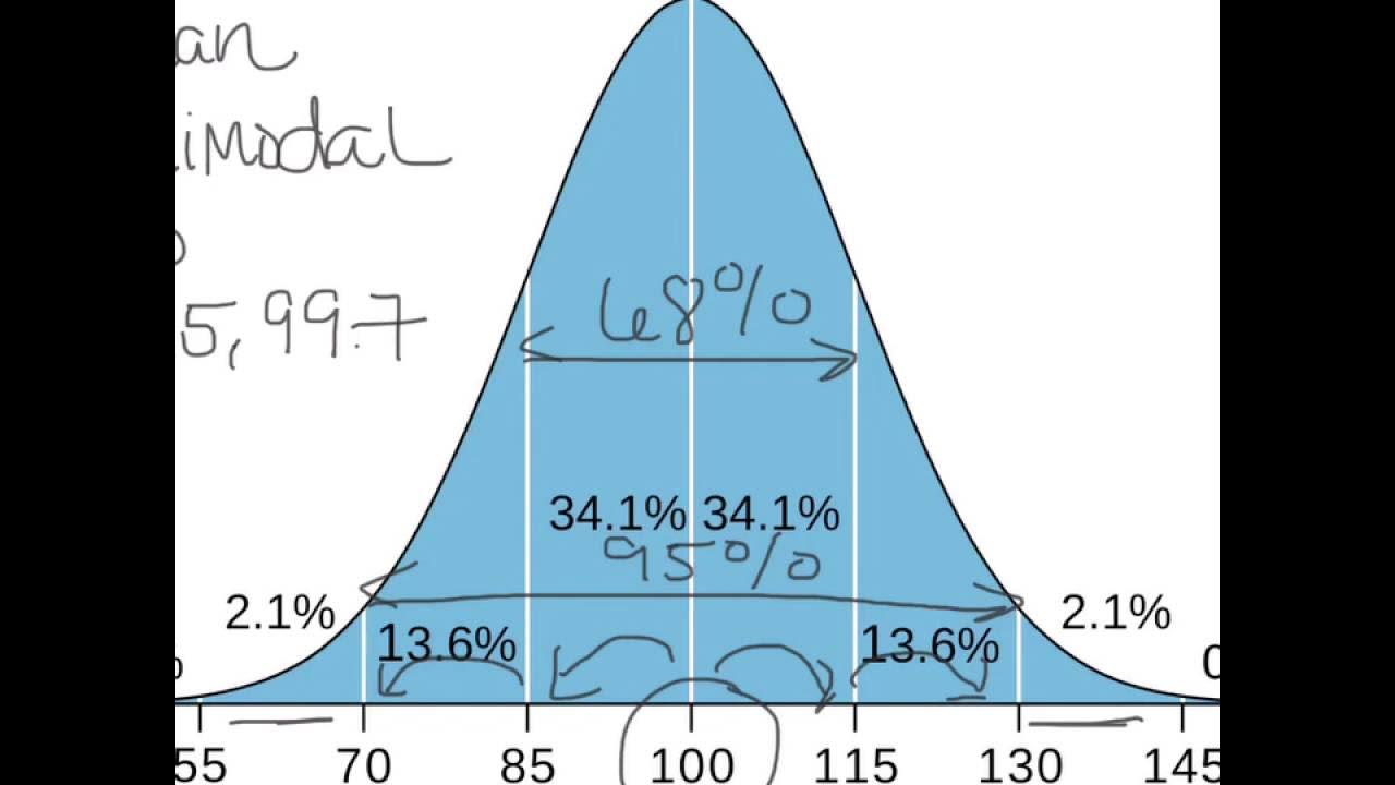
• 📊 The distribution under the curve is such that 34% of data is within one standard deviation on each side of the mean, 13.5% between one and two standard deviations, and 2.5% in the outermost tails.
• 👤 The Empirical Rule can be applied to any dataset where the mean (μ) and standard deviation (σ) are known, and the distribution is assumed to be normal.
• 🗂️ The Empirical Rule is particularly useful for creating a rough sketch of the histogram based on just two numerical values, enhancing our understanding of data distribution.

Q & A

What is the Empirical Rule?

The Empirical Rule is a guideline used to visualize the distribution of data when it is assumed to be bell-shaped or normally distributed. It states that approximately 68% of the data falls within one standard deviation of the mean, 95% within two standard deviations, and 99.7% within three standard deviations.

How does the Empirical Rule improve upon Chebyshev's Rule for normal distributions?

Chebyshev's Rule provides a rough estimate of data distribution for any dataset, but for normal distributions, it can be too broad. The Empirical Rule offers a more precise visualization of the distribution by using the specific properties of bell-shaped distributions, allowing for a more accurate representation based on the mean and standard deviation.

What percentage of data is expected to fall within one standard deviation of the mean in a normal distribution?

According to the Empirical Rule, approximately 68% of the data is expected to fall within one standard deviation of the mean in a normal distribution.

What does it mean for a distribution to be bell-shaped?

A bell-shaped distribution, also known as a normal distribution, is symmetrical and centered around the mean, with the data points decreasing in frequency as they move away from the mean, resembling the shape of a bell.

How can you determine the shape of the bell curve using the Empirical Rule?

By knowing the mean and standard deviation, you can determine the shape of the bell curve using the Empirical Rule. You plot the values at one, two, and three standard deviations from the mean and draw the curve with the appropriate slopes and widths to reflect the percentages of data within those ranges.

What percentage of the data is outside of three standard deviations in a normal distribution?

In a normal distribution, only about 0.3% of the data falls outside of three standard deviations from the mean.

How does the Empirical Rule help in visualizing the tails of a normal distribution?

The Empirical Rule helps visualize the tails of a normal distribution by indicating that 5% of the data is outside of two standard deviations and 32% is outside of one standard deviation. This information allows for the correct drawing of the tails with increasing slopes towards the center.

What is the significance of the percentages 34%, 13.5%, and 2.5% in the context of the Empirical Rule?

These percentages represent the distribution of data under the bell curve: 34% of the data is within one standard deviation on either side of the mean, 13.5% is between one and two standard deviations on either side, and 2.5% is outside of two standard deviations but within three standard deviations on either side.

Can the Empirical Rule be applied to any type of data distribution?

No, the Empirical Rule can only be applied to data distributions that can be assumed to be normal or bell-shaped. It does not apply to skewed or other non-normal distributions.

How can the Empirical Rule be validated using a real dataset?

The Empirical Rule can be validated by applying it to a dataset with a known mean and standard deviation and then comparing the predicted percentages within one, two, and three standard deviations to the actual data distribution, such as through a histogram.

What is the importance of knowing the mean and standard deviation in the context of the Empirical Rule?

Knowing the mean and standard deviation is crucial for the Empirical Rule because these two numbers alone enable the accurate visualization of the data's distribution shape, providing a clear understanding of how the data is spread around the mean.

Outlines

00:00

📊 Empirical Rule for Bell-Shaped Distributions

The paragraph introduces the Empirical Rule as a method to visualize data distribution when it can be assumed to be bell-shaped. It explains that unlike Chebyshev's Rule, which is applicable to any dataset, the Empirical Rule provides a more precise estimation for bell-shaped distributions. The rule states that approximately 68% of the data falls within one standard deviation of the mean, 95% within two standard deviations, and 99.7% within three standard deviations. An example is given with a mean of 50 and a standard deviation of 10, illustrating how observations are distributed around the mean. The significance of the Empirical Rule is highlighted in its ability to determine the shape of the bell curve using just the mean and standard deviation. The paragraph also describes how to sketch the bell curve based on these statistics, including the distribution of data within and outside standard deviations, and the proportion of data in the tails of the distribution.

Keywords

💡Chebyshev's Rule

Chebyshev's Rule is a statistical principle that provides a lower bound on the probability that a data point lies within a certain distance (k standard deviations) from the mean, regardless of the shape of the distribution. In the video, it is mentioned as a preliminary method to understand the distribution of data before moving on to more specific rules like the Empirical Rule. It's a general approach that does not assume a normal distribution, which is a key contrast to the Empirical Rule discussed later.

💡Empirical Rule

The Empirical Rule, also known as the 68-95-99.7 rule, is a guideline for the distribution of values in a dataset that is approximately normally distributed. It states that for such distributions, approximately 68% of the data falls within one standard deviation of the mean, 95% within two standard deviations, and 99.7% within three standard deviations. The Empirical Rule is central to the video's theme as it allows for a more precise visualization of data distribution when the normal distribution assumption holds.

💡Bell-shaped distribution

A bell-shaped distribution, also known as a normal distribution, is a type of continuous probability function that is symmetric around the mean and has a bell-shaped curve. This term is crucial to the video's narrative as it sets the stage for applying the Empirical Rule. The video explains that when a dataset can be assumed to have a bell-shaped distribution, the Empirical Rule provides a more accurate representation of the data's spread than Chebyshev's Rule.

💡Standard Deviation

Standard deviation is a measure of the amount of variation or dispersion in a set of values. A low standard deviation indicates that the values tend to be close to the mean, while a high standard deviation indicates that the values are spread out over a wider range. In the context of the video, standard deviation is essential for applying both Chebyshev's Rule and the Empirical Rule, as it helps determine the spread of the data around the mean.

💡Mean

The mean, often referred to as the average, is the sum of all values in a dataset divided by the number of values. It is a central value that represents the 'center' of the data. The video uses the mean as a reference point for applying the Empirical Rule, showing how data is distributed around this central value within different standard deviation intervals.

💡Observations

In the context of the video, 'observations' refers to the individual data points within a dataset. The Empirical Rule provides probabilities for the distribution of these observations relative to the mean and standard deviation. The video uses the term to illustrate how most observations fall within certain standard deviation intervals in a normal distribution.

💡Histogram

A histogram is a graphical representation of the distribution of data, where the data is 'binned' and the height of each bin represents the frequency of data points within that bin. The video mentions the importance of comparing the histogram with the theoretical distribution derived from the Empirical Rule to validate the assumption of normality and the accuracy of the rule.

💡Data Visualization

Data visualization involves the use of graphical representations to display information in a way that is easy to understand and interpret. The video emphasizes the importance of visualizing data using the Empirical Rule to better understand the distribution of a dataset, especially when it can be assumed to be normally distributed.

💡President's Age at Inauguration

This is an example dataset used in the video to illustrate the application of the Empirical Rule. By calculating the mean and standard deviation of the ages of U.S. presidents at inauguration, the video demonstrates how to apply the Empirical Rule to determine the distribution of this specific dataset, assuming normality.

💡Normal Distribution

A normal distribution, also known as a Gaussian distribution, is a continuous probability distribution that is symmetric about the mean and follows a bell-shaped curve. The video discusses the importance of assuming a normal distribution when applying the Empirical Rule, as this assumption allows for more accurate predictions about the spread of the data.

Highlights

Chebyshev's Rule provides a rough estimate of data distribution for any dataset.

The Empirical Rule is used for data that can be assumed to have a bell-shaped (normal) distribution.

The Empirical Rule improves upon Chebyshev's Rule for normal distributions.

The Empirical Rule states that 68% of observations are within one standard deviation of the mean.

95% of observations are within two standard deviations of the mean according to the Empirical Rule.

99.7% of observations are within three standard deviations of the mean in a bell-shaped distribution.

In an example with a mean of 50 and a standard deviation of 10, roughly 68% of data lies between 40 and 60.

Approximately 95% of the data falls between 30 and 70, with 99.7% between 20 and 80.

The Empirical Rule helps visualize the shape of the bell curve using just the mean and standard deviation.

The tails of the distribution are on the x-axis beyond three standard deviations, as only 0.3% of data is outside this range.

5% of the data falls outside two standard deviations, mostly concentrated between two and three standard deviations.

32% of data lies outside one standard deviation, with 68% of data within this range.

13.5% of the data lies between one and two standard deviations on each side of the mean.

The Empirical Rule can be applied to any dataset where normal distribution can be assumed, such as U.S. presidents' ages at inauguration.

When comparing the Empirical Rule prediction with actual data, the estimated bell curve is usually close to the actual histogram.

Transcripts

Previously, we learned how to get a rough shape of

the distribution from a given mean and standard

deviation using Chebyshev's Rule - which can be

applied for any dataset. Next, we will discuss the

Empirical rule that allows us to better visualize

the data if we can only assume that it has a bell

shaped distribution.

For normal, also known as bell shaped,

distribution's the Chebyshev's estimate is too

rough and can be improved. If the distribution of

the data set is or can be assumed to be

approximately normal or bell shaped we can apply

the Empirical rule which states the following.

Approximately 68% of observations of within

one standard deviation; approximately 95%

of observations are within two standard deviations;

and approximately 99.7% of

observations are within three standard deviations.

For example, when the mean is 50 and the standard

deviation is 10 roughly 68% of observations

are between 40 and 60; roughly 95% of

observations are between 30 and 70; and roughly

99.7% of observations

are between 20 and 80.

The significance of the Empirical rule is that it

enables us to determine the shape of the bell

curve from the mean and standard deviation only.

First, we're going to draw a horizontal axis and

label the values that are one, two, three standard

deviations away from the mean including the mean.

Since only 0.3% of the data

are outside of three standard deviations we

can draw the tails that are basically on the x-axis

outside of the three standard deviations away from

the mean. 5% of the data are outside of

two standard deviations so we can continue drawing

the tails towards the middle by increasing the

slope by a notch.

32% of the data are outside of one

standard deviation so we continue drawing the tails

towards the middle by increasing the slope by

another notch. 68% of the data are within

one standard deviation so we connect the tails

with a bell shaped middle part.

According to the Empirical rule, we have the

following distribution of data under the curve: the

middle 68% are evenly split into two halves

(34% each); 27% of

the data is between one and two standard

deviations away which means 13.5%

in each half; 5% of the data outside

of the two standard deviations is mainly

concentrated between two and three standard

deviations which means 2.5% in each tail.

We can do the same for any mu and sigma. For example,

when mu is 50 and sigma is 10 we get the following.

In the president's age at inauguration data set, the

mean is approximately 55 and the standard

deviations approximately 6.5. We can

compute how much of the data exactly are within

one, two, and three standard deviations from the

mean and validate the Empirical rule. Remember the

Empirical rule only applies when the data

distribution can be assumed normal.

So just based on the two numbers we would draw the

following scale and would imagine the following

shape of the distribution only assuming that the

president's ages are normally distributed.

If we superimpose the actual histogram we will be

able to see that we're not that far off.

We discussed the Empirical Rule as the way to try

visualizing the bell shaped data from a numerical

summary. The significance of the Empirical Rule is

that it produces a very accurate shape of the

histogram based on just two numbers - the mean and

standard deviation.