But what is a convolution?
Summary
TLDRThis script explores the concept of convolution, a mathematical operation used in various fields like image processing and probability theory. It explains how convolution combines two lists or functions, such as multiplying polynomials or analyzing dice probabilities, to yield new insights. The video also delves into the practical application of convolution in blurring images and detecting edges. Furthermore, it introduces a faster algorithm for computing convolutions using the Fast Fourier Transform (FFT), which is more efficient than traditional methods, especially for large datasets.
Takeaways
- 🔢 Convolution is a mathematical operation that combines two lists of numbers or functions to produce a new list or function. It's different from simple addition or multiplication.
- 🎲 The concept is introduced through the example of rolling dice to illustrate how the sums can be visualized and calculated using convolution.
- 📊 Convolution is widely used in various fields such as image processing, probability theory, and solving differential equations, including in the context of polynomial multiplication.
- 💡 The script explains that convolution can be visualized by aligning one list with a flipped version of the other and calculating the sum of products at different offsets.
- 🎛️ In probability, convolution helps calculate the probability of various outcomes when dealing with non-uniform distributions, like weighted dice.
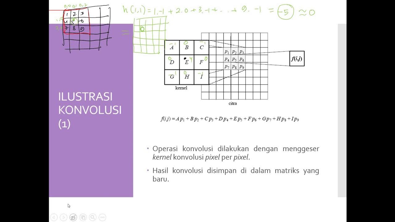
- 🖼️ In image processing, convolution is used for effects like blurring, edge detection, and sharpening by applying different 'kernels' or grids of values over the image.
- 📉 The script discusses how a moving average can be seen as a type of convolution, smoothing out data by averaging it within a sliding window.
- 🔄 The output length of a convolution is typically longer than the original lists, but in computer science, it can be truncated to match the original size.
- 🌀 The Fast Fourier Transform (FFT) algorithm is highlighted as a way to compute convolutions much more efficiently (O(n log n) instead of O(n²)) by leveraging the properties of polynomial multiplication.
- 🧮 An interesting connection is made to the idea that standard integer multiplication can also be viewed as a form of convolution, hinting at the possibility of more efficient multiplication algorithms for very large numbers.
Q & A
What are the three basic ways to combine two lists of numbers?
-The three basic ways to combine two lists of numbers are by adding them term by term, multiplying them term by term, and using a convolution, which is less commonly discussed but very fundamental.
How is convolution different from addition and multiplication of lists?
-Convolution is different from addition and multiplication of lists because it involves flipping one of the lists, aligning them at various offset values, taking pairwise products, and then summing them up, which creates a genuinely new sequence rather than just combining existing values.
In what contexts are convolutions commonly used?
-Convolution is ubiquitous in image processing, a core construct in probability theory, frequently used in solving differential equations, and is also seen in polynomial multiplication.
How does the concept of convolution relate to rolling dice and calculating probabilities?
-Convolution relates to rolling dice and calculating probabilities by visualizing the outcomes on a grid where diagonals represent constant sums, allowing for easy counting of combinations that result in a given sum.
What is the significance of the normal distribution in the context of probability as explained in the script?
-The normal distribution is significant in probability because it naturally aligns with the process of convolution, which is a fundamental way to calculate probabilities when dealing with non-uniform probabilities across different outcomes.
How does the script explain the concept of convolution in the context of image processing?
-The script explains convolution in image processing by using the example of blurring an image. It demonstrates how a grid of values (kernel) is used to multiply and sum pixel values, creating a smoothed or blurred version of the original image.
What is a kernel in the context of image processing?
-In image processing, a kernel is a small grid of values that is used to apply effects to an image through convolution. Different kernels can be used for various effects like blurring, edge detection, or sharpening.
How does the script connect the concept of convolution to polynomial multiplication?
-The script connects convolution to polynomial multiplication by showing that the process of creating a multiplication table for polynomials and summing along diagonals is equivalent to a convolution operation, which helps in expanding and combining polynomial terms efficiently.
What is the fast Fourier transform (FFT) and how does it relate to computing convolutions?
-The fast Fourier transform (FFT) is an algorithm that computes the discrete Fourier transform and its inverse very efficiently. It relates to computing convolutions by allowing the conversion of convolution operations into multiplications in the frequency domain, which can be computed much faster, especially for large lists.
How does the script suggest that the concept of convolution can be used to multiply large integers more efficiently?
-The script suggests that by treating large integers as coefficients of polynomials, sampling them at roots of unity, and using the FFT algorithm, it's possible to multiply the integers more efficiently with an algorithm that requires O(n log n) operations instead of the traditional O(n^2).
Outlines

Dieser Bereich ist nur für Premium-Benutzer verfügbar. Bitte führen Sie ein Upgrade durch, um auf diesen Abschnitt zuzugreifen.
Upgrade durchführenMindmap

Dieser Bereich ist nur für Premium-Benutzer verfügbar. Bitte führen Sie ein Upgrade durch, um auf diesen Abschnitt zuzugreifen.
Upgrade durchführenKeywords

Dieser Bereich ist nur für Premium-Benutzer verfügbar. Bitte führen Sie ein Upgrade durch, um auf diesen Abschnitt zuzugreifen.
Upgrade durchführenHighlights

Dieser Bereich ist nur für Premium-Benutzer verfügbar. Bitte führen Sie ein Upgrade durch, um auf diesen Abschnitt zuzugreifen.
Upgrade durchführenTranscripts

Dieser Bereich ist nur für Premium-Benutzer verfügbar. Bitte führen Sie ein Upgrade durch, um auf diesen Abschnitt zuzugreifen.
Upgrade durchführen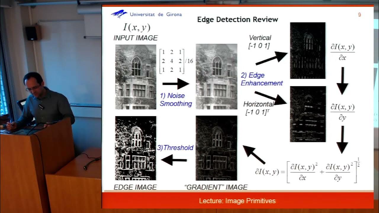


5.0 / 5 (0 votes)
