Overview of Differential Equations
Summary
TLDRThis video script introduces a series on ordinary differential equations, focusing on first and second order equations, which are fundamental in applications and often solvable. It covers linear and nonlinear equations, the significance of derivatives, and the role of inputs in systems like banking or springs. The script also touches on the challenges of solving higher order and nonlinear equations, the utility of eigenvalues and eigenvectors in systems of equations, and the prevalence of numerical solutions, highlighting MATLAB's ODE solvers. The goal is to provide a clear understanding of basic differential equations, with aspirations to eventually cover partial differential equations.
Takeaways
- 📚 The video series will focus on ordinary differential equations, particularly first and second order equations, which are most commonly seen in applications and can often be solved when possible.
- 🔍 First order equations involve first derivatives, representing the rate of change of the unknown function, often influenced by the function itself and external inputs.
- 📈 Linear equations are characterized by the presence of the unknown function y by itself, whereas nonlinear equations can involve more complex relationships like y squared or the sine of y.
- 🔬 Second order equations involve second derivatives, which relate to acceleration and the bending of the graph, a key concept in physics as described by Newton's laws.
- 🌐 Systems of equations are represented by vectors and matrices, where multiple equations are coupled, and eigenvalues and eigenvectors from linear algebra can simplify these by decoupling them into solvable individual equations.
- 📉 Linearity and constant coefficients are crucial for solving differential equations explicitly; without them, numerical methods become necessary.
- 🧬 Exponential functions are particularly important in differential equations, often leading to solutions that are also exponential and easily recognizable.
- 📝 Solutions to some differential equations may involve integrals of the function, requiring either lookup or numerical integration.
- 🔢 For completely nonlinear functions or equations with varying coefficients, numerical solutions are typically employed, which can be efficiently computed using software like MATLAB.
- 🛠 MATLAB's ODE solvers, starting with the simple Euler method and advancing to the more accurate ODE 45, are essential tools for finding numerical solutions to differential equations.
- 🎯 The ultimate goal of the series is to cover not only ordinary differential equations but also to introduce and explore partial differential equations, such as the heat, wave, and Laplace equations.
Q & A
What is the main topic of the first video in the series?
-The main topic of the first video is to provide an outline of what can be learned about ordinary differential equations, focusing on first and second order equations.
Why are first order differential equations important in applications?
-First order differential equations are important because they involve first derivatives, which represent the rate of change of an unknown function with respect to time, and they are often solvable when fortunate.
What does the term 'forcing term' refer to in the context of differential equations?
-In the context of differential equations, a 'forcing term' refers to an input function, denoted as q(t), that influences the system and becomes part of the solution y(t), causing it to grow, decay, or oscillate.
What is the difference between a linear and a nonlinear differential equation?
-A linear differential equation has terms where the unknown function y appears to the first power only, while a nonlinear differential equation has terms where y or its derivatives appear in a power higher than one or in a non-polynomial form.
How does the concept of 'mass' relate to second order differential equations in physics?
-In physics, particularly in Newton's law, the mass is a physical constant that multiplies the acceleration in a second order differential equation, representing the resistance to acceleration due to the object's inertia.
What is the significance of eigenvalues and eigenvectors in systems of differential equations?
-Eigenvalues and eigenvectors are significant in systems of differential equations because they simplify the problem by transforming a set of coupled equations into a set of uncoupled equations, making it easier to find solutions.
What numerical method does the script mention for solving differential equations?
-The script mentions the numerical method ODE 45 in MATLAB, which is a high-accuracy, flexible method for solving ordinary differential equations.
Who is credited with the simple numerical method mentioned in the script?
-Leonhard Euler is credited with the simple numerical method mentioned in the script, which is the basis for more advanced methods like ODE 45.
What are partial differential equations and how do they differ from ordinary differential equations?
-Partial differential equations (PDEs) involve partial derivatives and have multiple variables, unlike ordinary differential equations (ODEs) which typically involve a single independent variable. PDEs are used to describe phenomena in multiple dimensions, such as heat conduction or wave propagation.
What are the goals for the end of the series mentioned in the script?
-The goals for the end of the series are to reach and explain partial differential equations, including the heat equation, wave equation, and possibly the Laplace equation, providing a comprehensive understanding of differential equations beyond the basics.
Outlines

Dieser Bereich ist nur für Premium-Benutzer verfügbar. Bitte führen Sie ein Upgrade durch, um auf diesen Abschnitt zuzugreifen.
Upgrade durchführenMindmap

Dieser Bereich ist nur für Premium-Benutzer verfügbar. Bitte führen Sie ein Upgrade durch, um auf diesen Abschnitt zuzugreifen.
Upgrade durchführenKeywords

Dieser Bereich ist nur für Premium-Benutzer verfügbar. Bitte führen Sie ein Upgrade durch, um auf diesen Abschnitt zuzugreifen.
Upgrade durchführenHighlights

Dieser Bereich ist nur für Premium-Benutzer verfügbar. Bitte führen Sie ein Upgrade durch, um auf diesen Abschnitt zuzugreifen.
Upgrade durchführenTranscripts

Dieser Bereich ist nur für Premium-Benutzer verfügbar. Bitte führen Sie ein Upgrade durch, um auf diesen Abschnitt zuzugreifen.
Upgrade durchführenWeitere ähnliche Videos ansehen
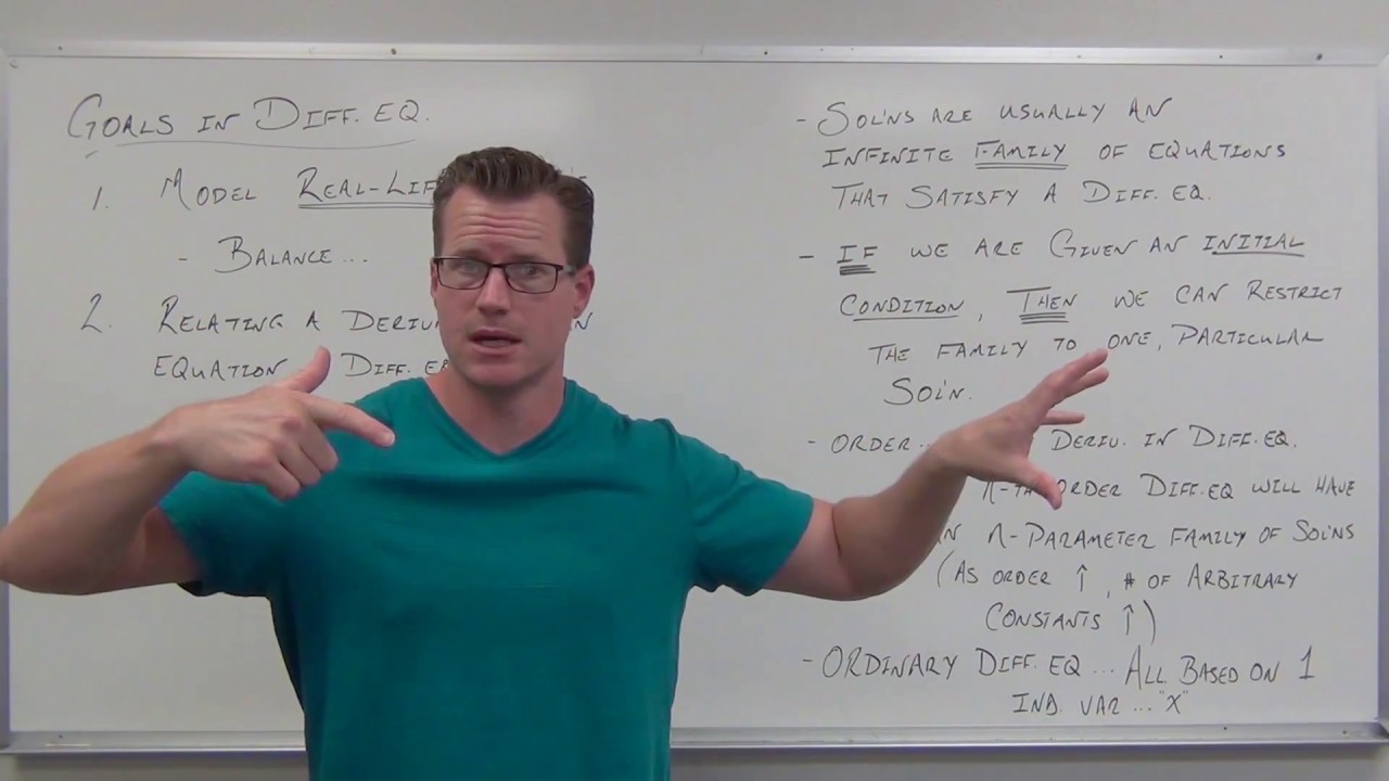
Introduction to Differential Equations (Differential Equations 2)
Fisika Komputasi - Metode Finite Difference 05 Sifat Diferensial dan Persamaan Diferensial

A concept of Differential Equation
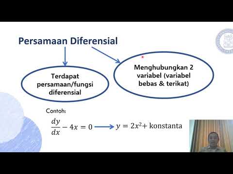
Pengantar Persamaan Diferensial
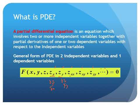
Persamaan Diferensial Parsial (Pengertian, Definisi, dan Klasifikasi)

Differential equations, a tourist's guide | DE1
5.0 / 5 (0 votes)
