43 R CNNs, SSDs, and YOLO

Summary

This video explores the evolution of object detection in computer vision, from traditional methods like HOG and SVM to deep learning approaches. It covers the breakthrough of R-CNNs, their evolution into Fast R-CNNs and Faster R-CNNs, and introduces Single Shot Detectors (SSDs) and the revolutionary YOLO algorithm. The video explains how these advanced detectors work, their speed and accuracy, and touches on metrics like Intersection over Union (IoU) and Mean Average Precision (mAP). It concludes with a look at the latest advancements in YOLO, setting the stage for implementing these detectors using Python and OpenCV.

Takeaways

• 🔎 **Object Detection Overview**: Object detection is a crucial part of computer vision that combines object classification and localization to identify and locate objects within images.
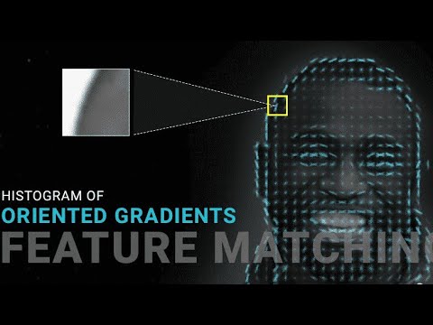
• 🐾 **Historical Context**: Early object detection methods like Haar cascade classifiers and Histogram of Gradients (HOG) with SVMs have been largely replaced by deep learning approaches due to their inefficiency with multiple object classes.
• 🚀 **Deep Learning Breakthrough**: In 2014, the introduction of Region-based Convolutional Neural Networks (R-CNNs) marked a significant advancement in object detection, achieving high performance in the PASCAL VOC challenge.
• 📈 **Selective Search Algorithm**: R-CNNs use selective search to propose regions of interest within an image, which are then classified by a CNN and refined using a linear regression for bounding boxes.
• 📏 **Intersection over Union (IoU)**: IoU is a metric used to evaluate the accuracy of object detection by measuring the overlap between the predicted bounding box and the ground truth.
• 🏎️ **Fast R-CNN**: An evolution of R-CNN, Fast R-CNN improved speed by reducing the need for multiple model training and execution, using region of interest (ROI) pooling.
• 🚀 **Faster R-CNN**: Building on Fast R-CNN, Faster R-CNN further increased speed by eliminating the need for selective search, thus speeding up the region proposal stage.
• 🏁 **Single Shot Detectors (SSDs)**: SSDs introduced multiscale features and default boxes to significantly increase detection speed, achieving near real-time performance with minimal accuracy loss.
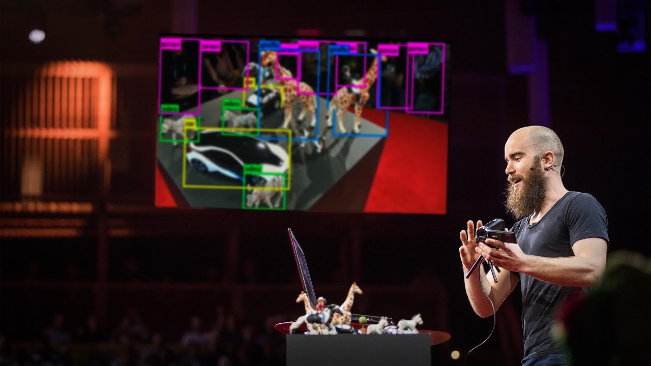
• 🌐 **YOLO (You Only Look Once)**: YOLO revolutionized object detection by using a single neural network applied to the full image, allowing for fast and efficient detection by predicting bounding boxes and class probabilities directly.
• 🏆 **YOLOv3**: The latest version of YOLO, YOLOv3, includes improvements like multi-scale training and batch normalization, enhancing its ability to detect objects of various sizes and resolutions.

Q & A

What is object detection in the context of computer vision?

Object detection is a crucial aspect of computer vision that combines object classification and localization. It not only identifies the presence of an object within an image but also determines the region or bounding box of the object, allowing for multi-class detection unlike earlier single-class detectors.

How do traditional non-learning methods for object detection compare to deep learning methods?

Traditional methods such as Haar cascade classifiers and Histogram of Gradients (HOG) with Linear SVMs are considered outdated compared to deep learning methods. Deep learning object detectors significantly outperform these traditional methods, offering better accuracy and applicability in a wider range of scenarios.

What was the breakthrough in deep learning object detection in 2014?

In 2014, the introduction of Regions with CNNs (R-CNNs) marked a significant breakthrough in deep learning object detection. R-CNNs achieved remarkably high performance in the PASCAL VOC challenge, a benchmark in computer vision for object detection.

How does the Selective Search algorithm contribute to object detection?

The Selective Search algorithm contributes to object detection by segmenting the image into different regions based on similarities in color or texture. It proposes regions of interest that are then passed through a CNN for classification, thus streamlining the process of generating bounding box proposals.

What is Intersection over Union (IoU) and why is it important in object detection?

Intersection over Union (IoU) is a metric used to measure the accuracy of an object detector by calculating the overlap between the predicted bounding box and the ground truth box. An IoU score above 0.5 is generally considered acceptable, indicating a good match between the predicted and actual object location.

How does the Mean Average Precision (mAP) metric help in evaluating object detectors?

Mean Average Precision (mAP) is a metric used to evaluate the performance of object detectors, especially when dealing with multiple detections for the same object. It provides a measure of accuracy by considering both the precision and recall of the detector across various classes of objects.

What improvements did Fast R-CNN bring over the original R-CNN?

Fast R-CNN improved upon the original R-CNN by reducing the computational overhead. It eliminated the need for separate models for feature extraction, classification, and bounding box regression by running the CNN only once over the entire image and then applying Region of Interest (ROI) pooling.

How do SSDs achieve near real-time performance in object detection?

SSDs (Single Shot MultiBox Detectors) achieve near real-time performance by using multiscale features and default boxes, which allow for efficient processing without the need for region proposal networks. They also reduce the resolution of images fed into the classifier, which contributes to their speed.

What is the core concept behind YOLO (You Only Look Once) object detection?

The core concept behind YOLO is to use a single neural network that processes the full image at once, allowing it to reason globally about the image content. It divides the image into a grid and predicts bounding boxes and class probabilities for each grid cell, which simplifies the detection process and enables fast performance.

How does YOLO's architecture differ from other object detection methods?

YOLO's architecture differs by using a single, unified model that combines region proposal, object recognition, and classification into one full convolutional neural network. This design allows for fast and efficient object detection without the need for multiple stages or models, which is a departure from methods like R-CNNs and SSDs.

Outlines

00:00

🔎 Introduction to Object Detection

This paragraph introduces the concept of object detection as the 'holy grail' of computer vision, emphasizing its importance in identifying and localizing multiple classes of objects within images. It contrasts single-class object detection with the more complex multi-class detection, highlighting the inefficiency of traditional methods like sliding windows. The paragraph also briefly mentions the advent of deep learning object detectors like R-CNNs, SSDs, and YOLO, which have revolutionized the field by offering efficient and accurate detection across various object classes.

05:01

📊 Understanding Object Detection Metrics

The second paragraph delves into the metrics used to evaluate object detection models, focusing on the Intersection over Union (IoU) metric. It explains how IoU measures the overlap between the predicted bounding box and the ground truth, with an IoU of over 0.5 being considered acceptable. The discussion includes the challenges of handling multiple bounding boxes for the same object and introduces the Mean Average Precision (mAP) metric as a way to assess model performance in such scenarios. The paragraph also touches on the evolution of deep learning object detectors, starting from R-CNNs to Fast R-CNNs and Faster R-CNNs, each improving upon the previous in terms of speed and efficiency.

10:02

🚀 Speeding Up Object Detection with SSDs

Paragraph three discusses the Single Shot Detectors (SSDs) and their significant improvement in speed over the R-CNN family, achieving near real-time performance. It explains how SSDs use multiscale features and default boxes, along with reduced image resolution for classification, to enhance speed without a substantial loss in accuracy. The paragraph also mentions the trade-off between increasing the number of default boxes for better accuracy and the consequent decrease in speed. The discussion concludes with an overview of SSD's structure, including the feature map extractor and the convolutional filter used for object detection.

15:03

🏆 The Rise of YOLO: Real-Time Object Detection

The final paragraph introduces the You Only Look Once (YOLO) object detection framework, which uses a single neural network applied to the full image, allowing for global reasoning and real-time detection. It outlines the evolution of YOLO from its initial version to YOLOv3, highlighting improvements such as batch normalization, higher resolution training, and multi-scale training to enhance the detection of smaller objects. The paragraph also provides a brief overview of YOLO's architecture, consisting of 24 convolutional layers followed by fully connected layers, and encourages viewers to read the original paper for a deeper understanding.

Keywords

💡Object Detection

Object detection is a fundamental concept in computer vision that involves identifying and locating objects within an image or video frame. It is described in the video as the 'holy grail' of computer vision, highlighting its significance. The video script mentions object detection in various contexts such as face, pedestrian, and vehicle detection, emphasizing its broad applications. Object detection is crucial as it not only classifies the objects but also localizes them within a frame, which is essential for tasks like autonomous driving or surveillance systems.

💡RCNNs (Regions with CNNs)

RCNNs, or Regions with CNNs, are a type of deep learning object detector that were a breakthrough in the field, achieving high performance in the PASCAL VOC challenge. The video script explains how RCNNs work by proposing bounding boxes and passing these to an image classifier. RCNNs were significant in advancing object detection by addressing the exhaustive search problem previously performed by sliding windows, thus improving efficiency and accuracy.

💡Selective Search

Selective Search is an algorithm used in the context of RCNNs to generate region proposals for object detection. The video script describes how it segments the image into different groups by combining similar areas such as colors or textures, which are then proposed as regions of interest. This process is crucial for RCNNs as it reduces the number of regions that need to be classified, thus improving the speed and efficiency of the object detection process.

💡CNNs (Convolutional Neural Networks)

CNNs are a class of deep learning models that are widely used in image recognition tasks, including object detection. The video script mentions how CNNs are used to classify the regions proposed by the Selective Search algorithm. CNNs are fundamental to the operation of RCNNs, as they extract features from the proposed regions and classify them, which is a critical step in the object detection pipeline.

💡SVM (Support Vector Machine)

SVM, or Support Vector Machine, is a machine learning algorithm used for classification tasks. In the context of the video, SVM is used after the CNN has extracted features from the regions proposed by Selective Search to classify the objects. The video script explains that the CNN features are fed into an SVM classifier, which then determines the class of the objects within the proposed regions.

💡Bounding Box

A bounding box is a rectangular frame that is used to localize an object within an image. The video script discusses how bounding boxes are proposed by the Selective Search algorithm and then refined by the CNN and SVM classifiers. Bounding boxes are essential in object detection as they provide the spatial information needed to identify the exact location of objects within an image.

💡Intersection over Union (IoU)

IoU, or Intersection over Union, is a metric used to evaluate the accuracy of object detection models. It is defined as the area of overlap between the predicted bounding box and the ground truth box, divided by the area of their union. The video script uses IoU to illustrate how well a predicted box aligns with the actual object's location. An IoU score over 0.5 is generally considered acceptable, indicating a good match between the predicted and true bounding boxes.

💡Faster R-CNN

Faster R-CNN is an evolution of the original RCNN, designed to improve speed and efficiency. The video script explains how Faster R-CNN addresses the slow performance of RCNNs by running the CNN across the entire image just once, using a technique called Region of Interest (ROI) pooling. This approach reduces the need for multiple passes and speeds up the object detection process.

💡SSD (Single Shot Detector)

SSD, or Single Shot Detector, is another deep learning object detector that is highlighted in the video script for its speed and efficiency. Unlike RCNNs, SSDs use multiscale features and default boxes, which allow them to operate at near real-time speeds with minimal loss in accuracy. The video script mentions SSDs in the context of their high frame rates and their ability to handle multiple objects and scales within an image.

💡YOLO (You Only Look Once)

YOLO, or You Only Look Once, is a state-of-the-art object detection algorithm that is praised in the video script for its speed and accuracy. YOLO operates by dividing the image into a grid and predicting bounding boxes and class probabilities for each grid cell. The video script describes YOLO's architecture and how it uses a single neural network applied to the full image, allowing for global reasoning and fast detection. YOLO's approach results in a balance between speed and accuracy, making it suitable for real-time applications.

Highlights

Introduction to deep learning object detectors like R-CNNs, SSDs, and YOLO.

Object detection is the 'holy grail' of computer vision, enabling multi-class detection.

Object detection combines classification and localization.

Traditional non-learning methods like HOG with SVM are outdated compared to deep learning detectors.

Deep learning object detectors are more efficient than sliding window approaches.

R-CNNs were a breakthrough in 2014, achieving high performance in the PASCAL VOC challenge.

Selective Search algorithm is used to generate region proposals for R-CNNs.

SVM is used to classify features extracted by CNNs in R-CNNs.

Linear regression is applied to refine the bounding boxes in R-CNNs.

Intersection over Union (IoU) is a key metric for evaluating object detection.

Mean Average Precision (mAP) is used to handle multiple detections of the same object.

Fast R-CNN improved the speed of R-CNNs by reducing the need for separate models.

Faster R-CNN further increased speed by eliminating the selective search bottleneck.

SSDs use multiscale features and default boxes for faster detection.

YOLO uses a single neural network applied to the full image for real-time object detection.

YOLO divides the image into an SxS grid and predicts bounding boxes and probabilities for each region.

YOLOv2 introduced batch normalization and was fine-tuned for higher resolutions.

YOLOv3 introduced multi-scale training for better detection of smaller objects.

SSDs and YOLO are currently among the top-performing object detectors.

Upcoming video will cover implementing object detection with SSDs and YOLO in Python using OpenCV.

Transcripts

hi and welcome to video where we take a

look at some deep learning

object detectors such as rcnns ssds

and yolo so let's start what exactly is

object detection well it is actually the

holy grail of computer vision

it allows us to do things like this and

you would have seen this before in our

face object detectors and pedestrian and

vehicle object detectors

in earlier videos however those were

limited to just

one class and if you were to add

multiple classes you would have to pile

on multiple object detections and that

would slow things down significantly

so we're taking a look at now some deep

learning some very advanced

object detectors that make things like

this possible this is pretty cool isn't

it

car dog horse person in the back over

here so what exactly is this now object

detection as i said in earlier chapters

is a mix of

object classification and localization

classification means determining what

the object is and localization means

identifying the region or the bounding

box of the object and it's used in face

detection quite often which we've seen

in previous chapters

now the difference with object detection

and classification

is that object detection doesn't just

tell you when an image contains a cat or

not but it actually tells you where the

cat order objects or

animals could be in the image so that's

pretty cool

now non-learning methods of object

detection included

what we discussed earlier which was

horror cascade classifiers and another

one we didn't discuss in earlier

chapters was histogram of gradients hog

with linear svms that support vector

machines it's a machine learning

classifier

and the reason we didn't discuss these

is because they are pretty much

outdated now because deep learning

object detectors

are significantly better and it can be

used in a wide variety of applications

that make it very powerful but the

reason why these aren't useful although

they are

technically very useful when you're

detecting just one object that's why

they're still very useful for face

detection

however when you try to apply this for

multiple objects

detectors it actually breaks down it

doesn't work too well and it can often

be quite slow and that's because it

involves

an approach called sliding windows where

you have to slide this window at various

scales across the image

and that's why it is not a very

efficient method

so in 2014 deep learning object

detectors had

a huge breakthrough with something

called regions with cnns or rcnns for

short

and this achieved remarkably high

performance in the pascal

voc challenge that is object detection

data set that has been used to compete

and score in computer vision journals

and researchers

to assess how good their object

detection methods are so basically

imagenet

variation of it and in 2014 as i said

our cnn's achieved remarkable success

now let's take a look at how our cnns

work so rcnn's attempted to solve the

exhaustive search problem

previously performed by sliding windows

by proposing

bounding boxes and passing these

extracted boxes to an image classifier

so now how do we get these bounding box

proposals and that's where we use an

algorithm called selective sig

so imagine we have an input image here

and we just extract

interesting regions here we send these

regions now to a cnn

to classify and then we get different

classifications of what it thinks it is

so now let's take a look at the

selective search algorithm

this attempts to segment the image into

different groups by combining

similar areas such as colors or textures

this could be

interpreted as blobs or contours and

proposes which of these regions

it is interesting using some of the

metrics within the classified algorithm

and it proposes these boxes here coming

out of this

segmentation type task and basically

feeds these

boxes here to the cnn to classify

one selective search found these

interesting boxes it takes these boxes

and passes it through the cnn as i said

before

one was trained on imagenet dataset so

with the imagenet dataset so it's

quite well tuned and well exposed to a

lot of data

and then what we do we don't actually

use the cnn directly for classification

all that we can

we then use the svm i said it's a

support vector machine classifier to

classify the cnn extracted features we

just compute the cnn features and feed

it into another classifier

and svm type classifier so after the

region proposal has been classified

we then use a simple linear regression

to generate a tighter bounding box

but what exactly makes a good box how do

we know

this box puzzle over this guy here is a

good box

now before we move on to other types of

deep learning object detectors

we're going to discuss some metrics and

how you assess object detectors

now this brings us to something called

intersection over union

or the iou metric so iou is defined as

the size of the union

over the size of the prediction box so

typically an iou over

0.5 is considered acceptable now let's

take a look at this metric in a little

bit more detail

imagine this green box over this car

here is our true

human labeled box to identify the car

remember

what we want in localized boxes we don't

want a box that predicts

half of the car and then it says at the

back wheel or we don't want a box that

covers

the car yes but covers a lot of extra

area around the car we want a box to be

nice and tight

exactly over the object in question that

we detected

so let's imagine this red box here is

the box

our object detector has proposed now it

looks fairly good it covers roughly

about 80 percent of the image

that's pretty good now let's take a look

at the one on the right

here this box which is actually covers a

lot more of the car covers almost 95

percent or more of the car

pretty much just missing out this little

little back piece here covers even more

so technically shouldn't this be

classified as a better box than this

well that's not exactly what we want

there is it

we don't want our box to be all over

here so that's how the iou metric

is developed it's the size of the union

over the size of the prediction box

so the union basically is this zone here

what is this zone here this zone is we

compute the area of this zone here

and the size of the prediction box is

put over here so

what we do okay this is the size

objection box is always going to be

bigger

so what this tells us is that we want

this prediction box

to cover as much of the green as

possible

without with being as small on the green

on the out as small as possible

over the green essentially hope you

understand that maybe i'm saying it

wrong

but essentially we just want this red

hair to cover

the green as much as possible without

being too

much over it or too much inside of it so

that's how we get this metric here

so anything over 0.5 is considered

fairly acceptable in my opinion

a lot of there are a lot more stricter

guidelines when it depends on type of

classifier you're building i mean

detective

but essentially 0.5 is a reasonable

score as you can see in this

box over here let's take a look at where

the iou would be

so the size of the union here looks

let's say estimated at 50 percent

maybe even a bit yeah 50 and then

besides the prediction box is definitely

maybe another 50 percent here

so you're going to end up with five

basically it's a fifty percent over a

hundred percent which is double the size

of this

so you're going to end up with something

like 0.5 whereas in this one

this one is basically you can say this

is 80 percent here

and this area that is on the outside is

probably like

0.6 of the ratio of this thing here so

you can understand how you get a much

higher iou

with this metric here now there's

another problem

when we have object vectors often times

we will have

multiple boxes being proposed over the

same object

and the object detector may not even

know it's doing it more than once

because remember it doesn't actually

know what's in the image it is

predicting interesting boxes in the

image

that it may or may not be correct it's

very hard to determine

for algorithm to determine is it two

cars packed side by side

is it one car so what we have to do is

if we have our ground shoot labels which

is the green

box here when we're testing our object

detectors you may often get

multiple windows proposed like this so

there's another metric called mean

average position or map for short

that we can use to get when we have

multiple boxes over the same thing

we can actually over the same true label

here ground truth

we can actually use this metric now to

determine the map score

and that determines the form of accuracy

of

our object detector so this one is

actually a bit confusing you can read

some pretty long blogs explaining this

metric that will help you understand

however for now just remember it's a

metric used to determine the performance

of

object detectors so now now that you

understand the metrics we can go back on

to the evolution of deep learning object

detectors

and let's take a look at something

called fast rcnn which is the evolution

of

our cnns by the same researchers and

what they did

they basically made some speed

improvements over the original rcnn

the original rcnn was quite slow because

it required three models to

train separately and use them in

conjunction when you're doing the

classification type work

execution in the end and this required

feature extraction

model an svm to predict a class and then

a linear regression to tighten the

bounding boxes in the end so you can see

in real time this would be quite slow so

fast rcnn solved this problem by

removing the overlap generated

now how what they did is that they ran

the scene and across the image just once

using a technique called

region of interest or roi pool so

essentially the problem the faster our

xenon solved was instead of running the

cnn

to extract features on all different

regions identified what they did sorry

they actually ran the cnn just once over

the entire image and then used those

features going forward into the second

and third

layers of models in the network so even

still that wasn't fast enough

and the researchers developed an even

faster rcnn and named it appropriately

faster or cnn however note there is no

fastest rcnn

just yet so what the researchers of the

microsoft research team did

to speed up our cnns or fast rcnns to

give it the faster flavor

was that they eliminated the bottleneck

that was involved when using selective

siege

so this sped up regent proposal

significantly as well

which now brings us to something called

single shot detectors or

ssds so we've just discussed and linked

the rcnn family and we've seen how

successful they can be and how they

evolved

however typically they still run at

roughly 7 frames per second

even on some fairly powerful hardware

however

ssds and even yellow are significantly

faster and you can actually see some of

the stats right here this is the fbs

as well you can see yellow and ssd is

topping the fps at 45 and 46 and you can

see the different scores

and in resolutions as well okay so how

did ssds improve speed so significantly

well

ssds use multiscale features and they

use something called default boxes

instead of looking at interesting

regions

and furthermore they actually dropped

resolution of the images that were fed

into the classifier itself

so this allowed ssds to achieve near

real-time speed performance

with almost no drop in accuracy and

sometimes they actually saw improved

accuracy when with well-trained ssds

so this is a general ssd structure it's

composed of two main parts

there's the feature map extractor and

vdd-16 was used

in the published paper but however

resonant and dead snap may provide

better results now

and then they used a convolutional

filter for the object detection part of

it

as well here so you can read the paper

in this link here if you want to get an

in-depth explanation of it but just to

summarize ssds are definitely faster

than faster rcnns however they are less

accurate in detecting

smaller objects now accuracy increases

if we increase the number of default

boxes

that allows us to get a more finer grid

on the image

however that actually slows down the

speed as well

and what it does with multi-scale

feature maps it allows it to improve the

optic detection

at various scales that's why we actually

can increase the accuracy

if we increase the density of the grid

so now

let's move on to yolo so the idea behind

yellow instead of using

a lot of different models and networks

and different

sections to do different things in the

object detector

yolo uses a single neural network that's

applied to the full image and this

allows yellow to reason about globally

across the image

when generating its predictions now it

is the direct development and evolution

of something called multibox

it basically takes multibox which was

used for region proposal

and turns it into object recognition and

then adds

a softmax layer in parallel with the box

regressor that combines everything into

a box classifier as well so you have the

entire object detector

built into it here so how it works it

divides the images into regions and

predicts boundary boxes and

probabilities for each region

so euler then uses a full convolutional

neural network allowing for inputs of

various sizes and i must say yolo is one

of the most impressive object detectors

that have

ever been built and so nice to use to

train

to evolve into different different

situations so now let's take a further

look at it and by the way if you want to

read and learn more about yolo you can

click this link here or go to the site

here to read the actual paper it's quite

good and actually

surprisingly entertaining as well so how

exactly does yolo work

well the image is firstly divided into

an s by s

grid and if the center of an object

falls into this grid cell

that cell is responsible for detecting

that object so let's say

this dog here falls into the center of

the cell here this cell is responsible

for

saying that this is a dog technically

however let's move on to the other steps

and you get a bigger picture of how it

works

so each grid then predicts a number of

bounding boxes and confidence scores for

those boxes and our confidence here is

defined

as the probability of an object

multiplied by the thresholded iu score

and iu scores of less than 0.5 are

typically just given a confidence

level of zero then by multiplying the

conditional

class probability and individual box

confidence predictions we get something

called the class specific confidence

score for each box

so you can see the steps here we have

all these bonding boxes here

you can see it proposes now a box region

around this dog here

and this is all based on the class

probability map and then once it gets

the final boxes here that it wants to

classify you can actually see the final

detections here

and the yellow is quite good and

effective in practice and quite

fast you can take a look at your

architecture here as well

or if you want as i said i encourage you

to read this paper here

now the architecture here has 24

convolutional

layers and followed by two fully

connected layers and

alternating one by one confidential

layers to reduce the feature spaces from

proceeding layers

now this may not make much sense to you

but you can read the paper to actually

understand the reasoning behind this

design

so let's talk about the evolution of

yolo now and was voted the people's

choice award people

at cvpr that's a big computer vision

conference

and then later on yellow vision 2 was

later released

and they were introduced batch

normalization which resulted in

improvements in the map score by two

percent and it was also fine-tuned to

work at higher resolutions

this is fairly high resolution for the

computer vision optic detection that is

working in real time i must say

and it gave a four percent increase in

map overall

yolo vision tree now was fine-tuned even

further and introduced multi-scale

training to help better detect smaller

objects

so this concludes our discussion on

yellow i hope you appreciated

what eola has brought to the table

yellow and ssds are basically neck and

neck

in the two best type of object detectors

out there

so now let's take a look at the summary

of what we just learned we learned

basically the evolution

of object detectors from hara cascade

classifiers and hogs

to the first deep learning object

detector which was our cnns then we

introduced fast rcnns and faster rcnns

we then explored single shot detectors

with ssds which are also quite good and

give quite good performance

and then we took a high level overview

of the yellow object detectors

where euler vision 3's latest one and

it's quite good right now

so now let's move on to the next video

where we start taking a look at

implementing object detection with

ssds and yolo in python using opencv 4.

so stay tuned thank you