Naive Bayes, Clearly Explained!!!

Summary

In this video, Josh Starburns introduces the concept of Naive Bayes classification, focusing on the Multinomial Naive Bayes Classifier. He explains its application in spam detection by calculating probabilities based on word frequency in normal and spam messages. Josh also covers key concepts like prior probability, likelihood, and how to overcome common issues like zero probabilities using smoothing techniques. Despite its simplicity, Naive Bayes proves highly effective in classifying messages. The video concludes with a discussion on why Naive Bayes is considered 'naive' and highlights additional resources for further study.

Takeaways

• 🤖 Naive Bayes is a classification technique used to predict outcomes based on word probabilities.
• 📊 A common version of Naive Bayes is the multinomial classifier, which is useful for text classification like spam filtering.
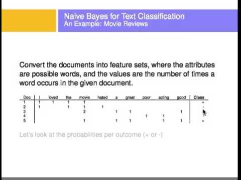
• 📈 The classifier works by creating histograms of words from normal and spam messages to calculate word probabilities.
• 📝 Probabilities of words appearing in normal or spam messages are used to predict if a new message is spam.
• 💡 Likelihoods and probabilities are interchangeable terms in Naive Bayes when dealing with discrete words.
• ⚖️ A prior probability is an initial guess about how likely a message is to be normal or spam, based on training data.
• 🔄 The Naive Bayes classifier treats word order as irrelevant, simplifying the problem but ignoring language structure.
• 🛠 A common problem, zero probability, is resolved by adding a count to each word's occurrences, known as 'smoothing'.
• 🚨 Naive Bayes is considered 'naive' because it assumes all features (words) are independent, ignoring relationships between them.
• 📚 Despite its simplicity, Naive Bayes often performs well in real-world applications, especially for tasks like spam filtering.

Q & A

What is the main focus of the video?

The video explains the Naive Bayes classifier, with a focus on the multinomial Naive Bayes version. It discusses how to use it for classifying messages as spam or normal.

What is the difference between multinomial Naive Bayes and Gaussian Naive Bayes?

Multinomial Naive Bayes is commonly used for text classification, while Gaussian Naive Bayes is used for continuous data like weight or height. The video focuses on the former and mentions that Gaussian Naive Bayes will be covered in a follow-up video.

How does Naive Bayes classify messages as normal or spam?

Naive Bayes calculates the likelihood of each word in a message being present in either normal or spam messages, multiplies these probabilities by initial guesses (priors) for each class, and compares the results to decide whether the message is normal or spam.

What is a 'prior probability' in the context of Naive Bayes?

A prior probability is the initial guess about the likelihood of a message being normal or spam, regardless of the words it contains. It is typically estimated from the training data.

Why is Naive Bayes considered 'naive'?

Naive Bayes is considered 'naive' because it assumes that all features (words in this case) are independent of each other. In reality, words often have relationships and specific orders that affect meaning, but Naive Bayes ignores this.

What problem arises when calculating probabilities for words not in the training data, and how is it solved?

If a word like 'lunch' does not appear in the training data, its probability becomes zero, which leads to incorrect classifications. This problem is solved by adding a small count (known as 'smoothing' or 'Laplace correction') to every word in the histograms.

How does Naive Bayes handle repeated words in a message?

Naive Bayes considers the frequency of words. For example, if a word like 'money' appears multiple times in a message, it increases the likelihood of the message being spam if 'money' is more common in spam messages.

What are 'likelihoods' in the Naive Bayes algorithm?

Likelihoods are the calculated probabilities of observing specific words in either normal or spam messages. In this context, likelihoods and probabilities can be used interchangeably.

How does Naive Bayes perform compared to other machine learning algorithms?

Even though Naive Bayes makes simplistic assumptions, it often performs surprisingly well for tasks like spam detection. It tends to have high bias due to its naivety but low variance, meaning it can be robust in practice.

What is the purpose of the alpha parameter in Naive Bayes?

The alpha parameter is used for smoothing to prevent zero probabilities when a word doesn't appear in the training data. In this video, alpha is set to 1, meaning one count is added to each word in the histograms.

Outlines

00:00

👨‍🏫 Introduction to Naive Bayes and Stack Quest

The narrator, Josh Starburns, introduces Stack Quest, a series that covers topics like Naive Bayes classification. He explains that the focus of this video is on the Multinomial Naive Bayes classifier, while the Gaussian version will be covered in another video. The concept of Naive Bayes is introduced through an example where messages from friends, family, and spam are filtered, and word probabilities are calculated.

05:00

📊 Calculating Probabilities for Normal and Spam Messages

The process of calculating word probabilities from histograms of normal and spam messages is discussed. Words like 'dear' and 'friend' are used to demonstrate how probabilities are assigned based on occurrences in normal messages. Similar calculations are made for spam messages.

Keywords

💡Naive Bayes

Naive Bayes is a type of probabilistic classifier based on applying Bayes' theorem with strong (naive) independence assumptions between the features. In the video, it is used to explain how this model helps classify whether messages are spam or normal by calculating probabilities based on word occurrences. The 'naive' aspect refers to the assumption that all features (words) are independent, which simplifies calculations but ignores word order.

💡Multinomial Naive Bayes

Multinomial Naive Bayes is a variant of Naive Bayes typically used for document classification, where features represent the frequencies of words. In this context, it is mentioned as the focus of the video, being applied to classify messages as spam or normal based on word probabilities. The video uses examples such as 'dear' and 'friend' to demonstrate how the model calculates probabilities based on word counts.

💡Gaussian Naive Bayes

Gaussian Naive Bayes is another variant of Naive Bayes, used when features follow a continuous distribution, typically a Gaussian (normal) distribution. It is briefly mentioned in the video as a follow-up topic and is contrasted with Multinomial Naive Bayes, which deals with discrete features like word counts.

💡Histogram

A histogram is a graphical representation that organizes a group of data points into specified ranges. In the video, histograms are used to show the frequency of words in normal and spam messages, helping calculate the probabilities of seeing each word in either category. These probabilities form the foundation of the Naive Bayes classification.

💡Prior Probability

Prior probability refers to the initial probability of a hypothesis before any evidence is considered. In the video, it represents the initial guess about whether a message is normal or spam before looking at specific words. For example, the prior probability that a message is normal is calculated based on the proportion of normal messages in the training data.

💡Likelihood

Likelihood refers to the probability of observing the data given a certain hypothesis. In this case, it is used to calculate the probability of encountering certain words given that the message is either normal or spam. The video clarifies that in this context, probabilities and likelihoods are interchangeable because the focus is on discrete word occurrences.

💡Spam Classification

Spam classification is the process of identifying whether a message is unsolicited or irrelevant. In the video, this is the main task the Naive Bayes model is being applied to, by calculating word probabilities and comparing them between normal and spam messages. Examples include calculating the probability of words like 'money' or 'dear' to classify new messages as spam or normal.

💡Alpha (Smoothing)

Alpha represents the smoothing parameter in Naive Bayes, often used to avoid zero probabilities for unseen words. The video explains that adding one to each word count (referred to as alpha = 1) prevents zero probabilities, ensuring that a message with unseen words like 'lunch' can still be classified correctly. This technique is crucial for improving the robustness of the model.

💡Bag of Words

The 'bag of words' model treats text as a collection of words, ignoring grammar and word order. In the video, this concept is emphasized when explaining how Naive Bayes is 'naive'—it assumes all words in a message are independent and order doesn't matter. Despite this simplification, the model can still perform well in classifying spam and normal messages.

💡Bias and Variance

Bias and variance are key concepts in machine learning that describe the trade-off between the accuracy of a model and its ability to generalize. The video explains that Naive Bayes has high bias because it ignores word order, but it also has low variance, meaning it performs consistently well in practice. This balance allows Naive Bayes to be effective despite its simplicity.

Highlights

Introduction to Naive Bayes and its application in spam filtering.

Multinomial Naive Bayes is the primary focus, with Gaussian Naive Bayes mentioned as a follow-up.

Example given of filtering messages by calculating probabilities of words in normal vs. spam messages.

Explanation of how histograms are used to calculate word probabilities for classification.

Clarification of probability vs. likelihood terminology.

Illustration of calculating the probability of the phrase 'dear friend' being in normal or spam messages.

The introduction of prior probability as an initial guess in Naive Bayes calculations.

Key calculation: 'Dear friend' is more likely to be a normal message based on computed probabilities.

Introduction of a problem when unseen words (like 'lunch') appear in new messages.

Solution to the zero-probability problem by adding a count (alpha) to each word.

Explanation of why Naive Bayes is called 'naive': it treats all word orders the same, ignoring grammar and syntax.

Even though Naive Bayes ignores word order, it performs well in practice for tasks like spam filtering.

Introduction of the terms 'high bias' and 'low variance' when describing Naive Bayes' effectiveness.

Promotion of StatQuest study guides for those preparing for exams or job interviews.

Final call to support StatQuest via Patreon, merchandise, or donations.

Transcripts

I'm at home during lockdown working on

my step quest yeah I'm at home during

lockdown working on my stack quest yeah

stack quest hello I'm Josh starburns

welcome to static quest today we're

gonna talk about naive Bayes and it's

gonna be clearly explained this stack

quest is sponsored by jad bio just add

data and their automatic machine

learning algorithms will do the rest of

the work for you for more details follow

the link in the pinned comment below

note when most people want to learn

about naive Bayes they want to learn

about the multinomial naive bayes

classifier and that's what we talk about

in this video

however just know that there is another

commonly used version of naive Bayes

called Gaussian naive Bayes

classification and I cover that in a

follow-up stat quest so check that one

out when you're done with this quest BAM

now imagine we received normal messages

from friends and family and we also

received spam unwanted messages that are

usually scams or unsolicited

advertisements and we wanted to filter

out the spam messages so the first thing

we do is make a histogram of all the

words that occur in the normal messages

from friends and family we can use the

histogram to calculate the probabilities

of seeing each word given that it was in

a normal message for example the

probability we see the word dear given

that we saw it in a normal message

is eight the total number of times deer

occurred in normal messages divided by

17 the total number of words in all of

the normal messages

and that gives us 0.47 so let's put that

over the word dear so we don't forget it

likewise the probability that we see the

word friend given that we saw it in a

normal message is 5 the total number of

times friend occurred in normal messages

divided by 17 the total number of words

in all of the normal messages and that

gives us zero point two nine so let's

put that over the word friend so we

don't forget it likewise the probability

that we see the word launch given that

it is in a normal message is 0.18

and the probability that we see the word

money given that it is in a normal

message is 0.06 now we make a histogram

of all the words that occur in the spam

and calculate the probability of seeing

the word dear given that we saw it in

the spam

and that is two the number of times we

saw deer in the spam divided by seven

the total number of words in the spam

and that gives us zero point two nine

likewise we calculate the probability of

seeing the remaining words given that

they were in the spam BAM now because

these histograms are taking up a lot of

space let's get rid of them but keep the

probabilities oh no it's the dreaded

terminology alert because we have

calculated the probabilities of discreet

individual words and not the probability

of something continuous like weight or

height these probabilities are also

called likelihoods

I mention this because some tutorials

say these are probabilities and others

say they are likelihoods in this case

the terms are interchangeable so don't

sweat it we'll talk more about

probabilities versus likelihoods when we

talk about Gaussian naive Bayes in the

follow-up Quest

now imagine we got a new message that

said dear friend and we want to decide

if it is a normal message or spam

we start with an initial guess about the

probability that any message regardless

of what it says is a normal message this

guess can be any probability that we

want but a common guess is estimated

from the training data for example since

8 of the 12 messages are normal messages

our initial guess will be 0.67 so let's

put that under the normal messages so we

don't forget it

oh no it's another dreaded terminology

alert the initial guests that we observe

a normal message is called a prior

probability

now we multiply the initial guess by the

probability that the word dear occurs in

a normal message and the probability

that the word friend occurs in a normal

message

now we just plug in the values that

we've worked out earlier and do the math

beep-boop beep-boop it and we get 0.09

we can think of 0.09 as the score that

dear friend gets if it is a normal

message however technically it is

proportional to the probability that the

message is normal given that it says

dear friend

so let's put that on top of the normal

messages so we don't forget

now just like we did before we start

with an initial guess about the

probability that any message regardless

of what it says is spam

and just like before the guests can be

any probability we want but a common

guess is estimated from the training

data

and since four of the twelve messages

are spam our initial guess will be 0.33

so let's put that under the spam so we

don't forget it

now we multiply that initial guess by

the probability that the word dear

occurs in spam and the probability that

the word friend occurs in spam

now we just plugged in the values that

we worked out earlier and do the math

BIP BIP BIP BIP BIP and we get 0.01

like before we can think of 0.01 as the

score the dear friend gets if it is spam

however technically it is proportional

to the probability that the message is

spam given that it says dear friend

and because the score we got for normal

message 0.09 is greater than the score

we got for spam 0.01 we will decide that

dear friend is a normal message double

BAM now before we move on to a slightly

more complex situation let's review what

we've done so far we started with

histograms of all the words in the

normal messages and all of the words in

the spam then we calculated the

probabilities of seeing each word given

that we saw the word in either a normal

message or spam then we made an initial

guess about the probability of seeing a

normal message

this guest can be anything between zero

and one but we based hours on the

classifications in the training data set

then we made the same sort of guess

about the probability of seeing spam

then we multiplied our initial guests

that the message was normal by the

probabilities of seeing the words dear

and friend given that the message was

normal then we multiplied our initial

guests that the message was spam by the

probabilities of seeing the words dear

and friend given that the message was

spam

then we did the math and decided that

dear friend was a normal message because

0.09 is greater than 0.01

now that we understand the basics of how

naive Bayes classification works let's

look at a slightly more complicated

example

this time let's try to classify this

message lunch money money money money

note this message contains the word

money four times and since the

probability of seeing the word money is

much higher in spam than in normal

messages then it seems reasonable to

predict that this message will end up

being spam so let's do the math

calculating the score for a normal

message works just like before we start

with the initial guess then we multiply

it by the probability we see lunch given

that it is in a normal message and the

probability we see money four times

given that it is in a normal message

when we do the math we get this tiny

number

however when we do the same calculation

for spam we get zero

this is because the probability we see

lunch in spam is zero since it was not

in the training data and when we plug in

zero for the probability we see lunch

given that it was in spam then it

doesn't matter what value we picked for

the initial guess that the message was

spam and it doesn't matter what the

probability is that we see money given

that the message was spam because

anything times zero is zero

in other words if a message contains the

word lunch it will not be classified as

spam and that means we will always

classify the messages with lunch in them

as normal no matter how many times we

see the word money

and that's a problem

to work around this problem people

usually add one count represented by a

black box to each word in the histograms

note the number of counts we add to each

word is typically referred to with the

Greek letter alpha in this case alpha

equals one but we could have said it to

anything

anyway now when we calculate the

probabilities of observing each word

we never get 0 for example the

probability of seeing lunch given that

it is in spam is 1/7 the total number of

words in spam plus for the extra counts

that we added

and that gives us 0.09 note adding

counts to each word does not change our

initial guess that a message is normal

or the initial guess that the message is

spam because adding a count to each word

did not change the number of messages in

the training data set that are normal or

the number of messages that are spam

now when we calculate the scores for

this message we still get a small number

for the normal message

but now when we calculate the value for

spam we get a value greater than zero

and since the value for spam is greater

than the one for a normal message we

classify the message as spam spam

now let's talk about why naive Bayes is

naive the thing that makes naive Bayes

so naive is that it treats all word

orders the same for example the normal

message score for the phrase dear friend

is the exact same for the score for

friend dear in other words regardless of

how the words are ordered we get 0.08

treating all word orders equal is very

different from how you and I communicate

every language has grammar rules and

common phrases but naivebayes ignores

all of that stuff

instead naivebayes treats language like

it is just a bag full of words and each

message is a random handful of them

naive bayes ignores all the rules

because keeping track of every single

reasonable phrase in a language would be

impossible that said even though naive

bayes is naive it tends to perform

surprisingly well when separating normal

messages from spam

in machine learning lingo we'd say that

by ignoring relationships among words

naivebayes has high bias but because it

works well in practice naive Bayes has

low variance shameless self-promotion

if you are not already familiar with the

terms bias and variance check out the

quest the link is in the description

below

triple spam

oh no it's one last shameless

self-promotion one awesome way to

support stack quest is to purchase the

naivebayes

stack quest study guide it has

everything you need to study for an exam

or job interview it's eight pages of

total awesomeness and while you're there

check out the other stack quest study

guides there's something for everyone

hooray we've made it to the end of

another exciting stat quest if you liked

this stack quest and want to see more

please subscribe and if you want to

support stack quest consider

contributing to my patreon campaign

becoming a channel member buying one or

two of my original songs or a t-shirt or

a hoodie or just donate the links are in

the description below alright until next

time quest on