The Normal Distribution and the 68-95-99.7 Rule (5.2)

Summary

This video script explores the concept of the normal distribution, also known as the bell curve, and its characteristics, including the role of population parameters like mean (μ) and standard deviation (σ). It explains the 68-95-99.7 rule, which approximates the distribution's area within one, two, or three standard deviations from the mean. The script uses practical examples like exam scores and heights to illustrate these principles, offering viewers a clear understanding of how data clusters around the central value and the distribution's spread.

Takeaways

• 📚 A parameter is a number that describes a population, while a statistic describes a sample. For example, the population mean is denoted by the Greek letter mu (μ), and the sample mean by x-bar (𝑥̄).
• 📊 The normal distribution, also known as the bell curve, is a symmetrical density curve that shows data clustering around a central value, the population mean.
• 🌟 The position of the normal distribution on the number line is determined by the population mean (μ), while the spread is determined by the population standard deviation (Σ).
• 📉 The larger the standard deviation (Σ), the more spread out the normal distribution becomes, and the flatter the curve. Conversely, a smaller standard deviation results in a less spread out, taller curve.
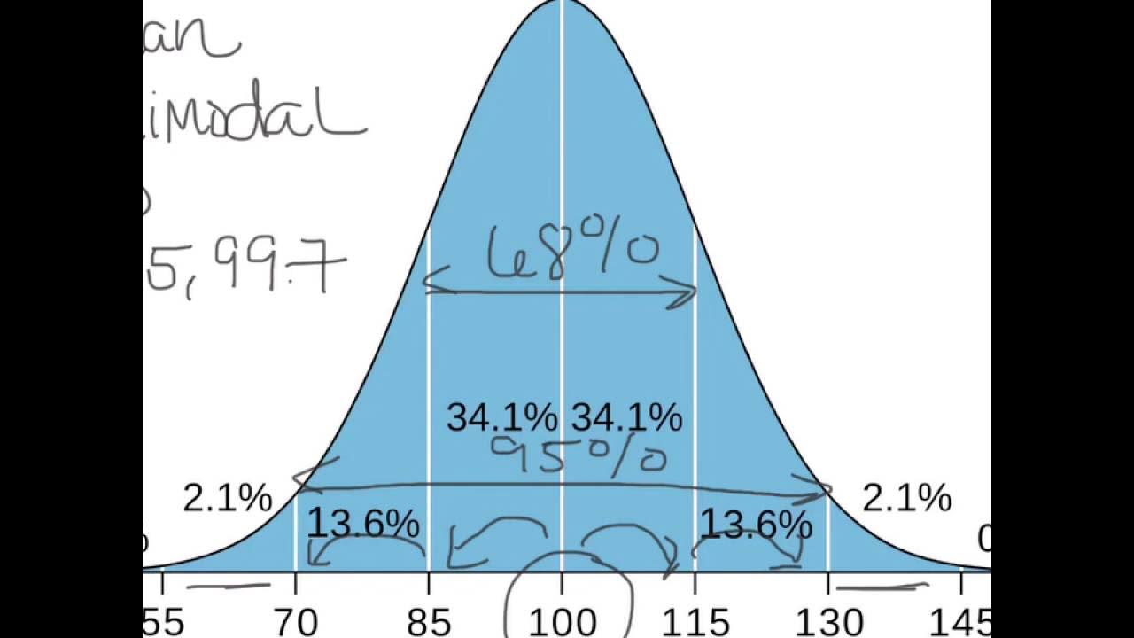
• 🔍 The normal distribution is unimodal and symmetric, meaning it has a single peak and can be divided into two equal halves around the mean.
• 📈 The 68-95-99.7 rule states that approximately 68% of data falls within one standard deviation of the mean, 95% within two standard deviations, and 99.7% within three standard deviations.
• 🚫 A normal distribution never touches the x-axis, extending infinitely in both directions, but the area beyond three standard deviations becomes very small.
• 📐 The normal distribution's shape and spread are characterized by two parameters: the mean (μ) and the standard deviation (Σ), and it can be denoted as X ~ N(μ, Σ²).
• 📝 The 68-95-99.7 rule can be applied to any normal distribution to approximate the areas under the curve, regardless of its specific shape or size.
• 📑 The script provides examples and practice questions to illustrate the application of the normal distribution and the 68-95-99.7 rule in calculating areas under the curve.
• 💻 For further learning, the video suggests visiting the website simpleearningpower.com for study guides and practice questions related to the normal distribution.

Q & A

What is the difference between a parameter and a statistic?

A parameter is a number that describes data from a population, while a statistic is a number that describes data from a sample.

What symbols are used to represent the sample mean and sample standard deviation?

The sample mean is represented by x-bar (x̄) and the sample standard deviation is represented by s.

What symbols are used to represent the population mean and population standard deviation?

The population mean is represented by the Greek letter mu (μ) and the population standard deviation is represented by the Greek letter sigma (σ).

What is a normal distribution and why is it sometimes called the bell curve?

A normal distribution is a special type of density curve that is bell-shaped. It is called the bell curve because of its shape.

How does the population mean (mu) affect the position of the normal distribution?

The population mean (mu) determines the position of the normal distribution. If the mean increases, the curve shifts to the right; if the mean decreases, the curve shifts to the left.

How does the population standard deviation (sigma) affect the spread of the normal distribution?

The population standard deviation (sigma) determines the spread of the normal distribution. A larger standard deviation results in a more spread-out distribution, while a smaller standard deviation results in a less spread-out distribution.

What does the notation N(μ, σ) mean in the context of a normal distribution?

The notation N(μ, σ) indicates that the variable X follows a normal distribution with a mean of μ and a standard deviation of σ.

What does the 68-95-99.7 rule state?

The 68-95-99.7 rule states that in a normal distribution, approximately 68% of the data falls within one standard deviation of the mean, 95% falls within two standard deviations, and 99.7% falls within three standard deviations.

If the mean height of students at a university is 5.5 feet with a standard deviation of 0.5 feet, what percentage of students are between 5 and 6 feet tall?

Approximately 68% of students are between 5 and 6 feet tall, according to the 68-95-99.7 rule.

In a normal distribution with a mean of 70 and a standard deviation of 10, what is the approximate area contained between 70 and 90?

The approximate area contained between 70 and 90 is 47.5%, as it represents half of the area within two standard deviations (95%).

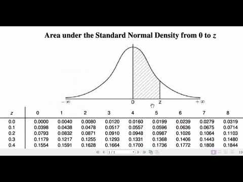
For a normal distribution with a mean of 0 and a standard deviation of 1, what is the approximate area contained between -2 and 1?

The approximate area contained between -2 and 1 is 81.5%, calculated by adding 47.5% (area from -2 to 0) and 34% (area from 0 to 1).

Outlines

00:00

📚 Introduction to Normal Distribution and Parameters vs. Statistics

This paragraph introduces the concept of the normal distribution, also known as the bell curve, which is a symmetrical density curve that represents data clustering around a central value, the population mean (μ). It distinguishes between parameters, which are characteristics of a population (e.g., μ and population standard deviation, Σ), and statistics, which describe sample data (e.g., sample mean, x-bar, and sample standard deviation, s). The paragraph also explains the significance of the mean and standard deviation in determining the position and spread of the normal distribution curve.

05:01

📊 Understanding the 68-95-99.7 Rule in Normal Distribution

The second paragraph delves into the 68-95-99.7 rule, which is a statistical principle used to approximate the distribution of data in a normal distribution. It states that approximately 68% of the data falls within one standard deviation of the mean, 95% within two standard deviations, and 99.7% within three standard deviations. The paragraph uses the example of student heights to illustrate this rule, explaining how the areas under the normal distribution curve correspond to percentages of the population. It also addresses the infinite nature of the normal distribution, which never touches the x-axis and extends indefinitely, and the diminishing areas beyond three standard deviations from the mean.

Keywords

💡Normal Distribution

Normal distribution, also known as Gaussian distribution, is a probability distribution that is characterized by its symmetric bell-shaped curve. In the video, it is described as a way to represent data that naturally clusters around a central value, which is the population mean. It is a fundamental concept in statistics and is used to model a wide range of phenomena in the natural and social sciences.

💡68-95-99.7 Rule

The 68-95-99.7 rule, also known as the empirical rule, is a quick way to approximate the proportion of data that falls within a certain number of standard deviations from the mean in a normal distribution. The video explains that about 68% of data falls within one standard deviation of the mean, 95% within two, and 99.7% within three, which is crucial for understanding the spread of data in normally distributed populations.

💡Parameter

A parameter is a numerical value that describes a characteristic of a population. In the context of the video, parameters are used to define the population mean (mu) and the population standard deviation (Sigma). These parameters are essential for understanding the overall characteristics of the population from which a sample is drawn.

💡Statistic

A statistic is a numerical value that describes a characteristic of a sample, which is a subset of the population. The video mentions sample mean (x-bar) and sample standard deviation (s) as examples of statistics. These are used to estimate the parameters of the population based on the sample data.

💡Bell Curve

The term 'bell curve' is synonymous with the normal distribution due to its characteristic shape. The video uses this term to illustrate the distribution's tendency to have most data points near the central value, with fewer data points as you move further away from the mean, creating a symmetrical, bell-shaped graph.

💡Population Mean (mu)

The population mean (mu) is the average value of a population and is represented by the Greek letter 'mu' in the video. It is a key parameter that determines the central location of the normal distribution curve. The video explains that increasing or decreasing the mean will shift the curve to the right or left, respectively.

💡Population Standard Deviation (Sigma)

The population standard deviation (Sigma) measures the amount of variation or dispersion in a set of values in a population. The video describes how a larger Sigma results in a more spread out distribution, while a smaller Sigma results in a distribution that is more concentrated around the mean.

💡Density Curve

A density curve is a graphical representation used in statistics to show the distribution of data. In the context of the video, the normal distribution is a type of density curve that must have a total area under the curve equal to one, reflecting the total probability of all possible outcomes.

💡Symmetric

Symmetry in the context of the normal distribution means that the curve is mirrored around the vertical line passing through the mean. The video explains that this symmetry allows the distribution to be divided into two equal halves, which is a key characteristic of normal distributions.

💡Unimodal

The term 'unimodal' refers to a distribution that has a single peak. The video mentions that the normal distribution is unimodal, indicating that it has one central peak around which the data is clustered, which is a defining feature of this type of distribution.

💡Empirical Rule

The empirical rule is another term for the 68-95-99.7 rule mentioned in the video. It provides a quick method to estimate the proportion of data within certain intervals in a normal distribution. The video uses this rule to demonstrate how to approximate the areas under the normal distribution curve.

Highlights

The video explains the concept of the normal distribution and the 68-95-99.7 rule.

Distinguishes between a parameter and a statistic, with examples of mean and standard deviation.

Clarifies the use of symbols x-bar for sample mean and s for sample standard deviation.

Describes the Greek letters mu and Sigma as symbols for population mean and standard deviation.

Explains the bell-shaped curve of the normal distribution and its relation to data clustering around the mean.

Discusses the natural occurrence of the normal distribution in variables such as height, weight, and blood pressure.

Illustrates how the population mean (mu) determines the position of the normal distribution.

Describes the role of the population standard deviation (Sigma) in the spread of the normal distribution.

Explains the effect of standard deviation on the shape of the normal distribution curve.

States that the normal distribution is unimodal and symmetric about its mean.

Details the notation for a normally distributed population with mean mu and standard deviation Sigma.

Introduces the 68-95-99.7 rule for approximating the areas under the normal distribution curve.

Demonstrates the application of the 68-95-99.7 rule using an example of students' heights.

Clarifies that the normal distribution extends to infinity and does not touch the x-axis.

Provides practice questions to apply understanding of the normal distribution and the 68-95-99.7 rule.

Shows how to calculate the area between specific values using the 68-95-99.7 rule.

Encourages viewers to support the channel for more educational content.

Directs viewers to the website for additional study guides and practice questions.

Transcripts

in this video we'll be learning about

the normal distribution and the 6895

99.7 rule when we talk about normal

distributions we refer to data we get

from a population or sample so before we

actually talk about the normal

distribution we need to first

distinguish the difference between a

parameter and a statistic a parameter is

a number that describes the data from a

population whereas a statistic is a

number that describes the data from a

sample examples of parameters and

statistics are the mean and standard

deviation but because of the definitions

we just talked about we have to be very

careful with what symbols we use to

represent these numbers when we are

dealing with a sample we use the symbol

x-bar to represent the sample mean and

we use the letter s to represent the

sample standard deviation these are

statistics when we are dealing with a

population we use the Greek letter mu to

represent the population mean and we use

the Greek letter Sigma to represent the

population standard deviation these are

parameters the population parameters mu

and Sigma are very important when we

talk about normally distributed

populations so what is a normal

distribution anyways a normal

distribution is a special type of

density curve that is bell-shaped for

this reason the normal distribution is

sometimes called the bell curve or the

normal curve the normal distribution

describes the tendency for data to

cluster around a central value in fact

this central value is the population

mean mu which is always located in the

middle of the curve so for any normal

distribution we can say that some data

points will fall below the mean other

data points will fall above the mean but

most of the data values are located near

the mean the normal distribution and its

shape actually arises from many

different variables found in nature such

as weight height volume blood pressure

and many more this is why the normal

distribution is commonly studied for

example exam scores are known to follow

a normal distribution

some people do great on exams some

people do poorly on exams but a large

majority of people score near the

average or the mean in this example the

average exam score is 50

because it is located in the middle of

the curve now that you know what a

normal distribution looks like we need

to talk about the population mean meal

and the population standard deviation

Sigma

both of these tell us important

information about how the normal

distribution looks we all talk about the

population mean mu first the population

mean mu characterizes the position of

the normal distribution if you increase

the mean the curve will follow and move

towards the right and if you decrease

the mean the curve will still follow and

move towards the left this happens

because the data will always cluster

around the mean in normally distributed

populations as a result the value of the

mean determines the position of the

normal distribution on the other hand

the population standard deviation Sigma

characterizes the spread of the normal

distribution the larger the standard

deviation the more spread out the

distribution will be and the smaller the

standard deviation the less spread order

will be notice that when the spread

increases the curve gets much flatter

and when the spread decreases the curve

gets taller the reason for this is

because the normal distribution is a

density curve and the total area of any

density curve must remain equal to one

or a hundred percent so changes in the

width of the curve must be compensated

for by changes in the height of the

curve and vice versa overall here are

some points about the normal

distribution the normal distribution is

unimodal this means that the

distribution has a single peak the

normal curve is symmetric about its mean

so you can clearly see that the

distribution can be cut into two equal

halves the parameters mu and Sigma

completely characterized the normal

distribution the population mean mu

determines the location of the

distribution and where the data tends to

cluster around the population standard

deviation Sigma determines how spread

out the distribution will be the

notation given to a population that

follows a normal distribution can be

written like this although it looks

scary it means what it says for the

variable X it follows a normal

distribution and has the mean mu with a

standard deviation of Sigma now that

you've been introduced to the normal

distribution

we can talk about the 6895 99.7 rule if

we were measuring the heights of all

students at a local university and found

that it was normally distributed with a

mean height of 5.5 feet and a standard

deviation of half a foot or 0.5 we can

construct a normal distribution as

follows

from here we can create intervals that

increase by the standard deviation so

we'll have six six point five and seven

and on the other side we'll have five

four point five and four so what the 68

95 99 point seven rule says is that

within one standard deviation away from

the mean it contains a total area of

zero point six eight or 68% because of

this we can say that 68% of the

population are between five and six feet

tall and if he go to standard deviations

away from the mean it contains an area

of 95 percent this means that 95 percent

of the people in the population have a

height between four point five and six

point five feet and finally within three

standard deviations away from the mean

it contains a total area of ninety-nine

point seven percent this means that for

the population we are studying

ninety-nine point seven percent of the

people are between four and seven feet

tall now you might be wondering what

happens if we go four standard

deviations away from the mean or five or

six standard deviations away from the

mean and to answer that you actually can

a normal distribution actually never

touches the x-axis it continues on to

infinity so you can go as many standard

deviations away from the mean as you

want but the area contained within these

regions will be very very small

the 6895 99.7 rule is a great way for

approximating the areas of a normal

distribution and this works for any

normal distribution no matter what shape

and size so let's do some practice

questions feel free to pause the video

at any point so you can try these

questions for yourself

question number one the normal

distribution below has a standard

deviation of 10 approximately what area

is contained between 70 and 90

in this question we know that the

population mean is equal to 70 because

it's in the center of the distribution

we also know from the question that one

standard deviation is equal to 10 and we

can see this because each interval goes

up by 10 according to the 6895 99.7 rule

we know that there is an area of 95

percent contained within two standard

deviations of the mean

two standard deviations to the right

gets us to 90 and two standard

deviations to the left gets us to 50

according to the 68 95 99 point 7 rule

this means that there is an area of 95

percent contained within this interval

however we are only interested in the

area from 70 to 90 so dividing this area

by two gives us our area of interest

95 percent divided by two gives us an

area of forty seven point five percent

and that is our answer question number

two for the normal distribution below

approximately what area is contained

between negative two and one in this

example we know that we have am u of

zero because zero is in the center of

the distribution and we know that we

have a sigma of one because each

interval goes up by one to approximate

the area between negative two and one we

use the 6895 99.7 rule we can

strategically divide this area into two

parts so that we can easily incorporate

this rule we'll start with the right

half which goes from zero to one we know

that one standard deviation away from

the mean gives us 68% and half of this

is 34% giving us our area from zero to

one the next half goes from zero to

negative two but we know that within two

standard deviations from the mean we

have an area of 95% dividing this by two

gives us the area from zero to negative

two which is equal to forty seven point

five percent and finally to get that

total area contained between negative

two and one

all we have to do is add these two areas

together and when we do we get a total

area of 81.5% if you found this video

helpful consider supporting us on

patreon to help us make more videos you

can also visit our website at simple

earning power com to get access to many

study guides and practice questions

thanks for watching