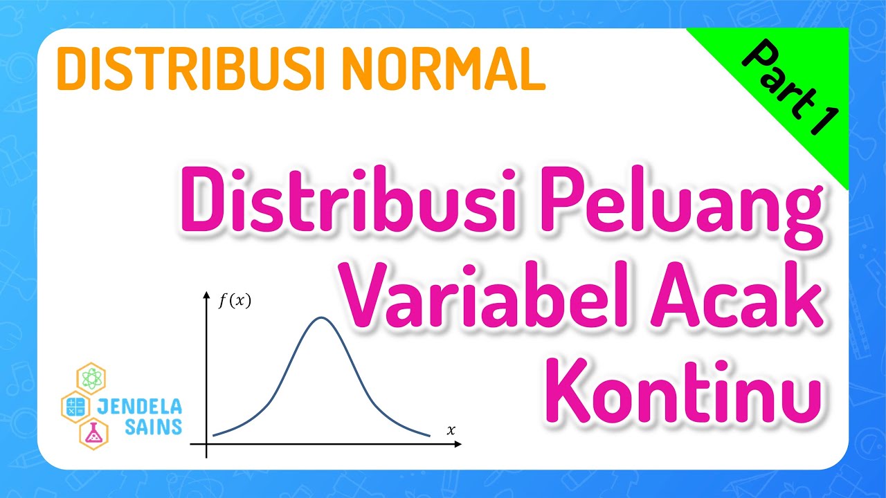
FRM: Normal probability distribution

Summary

David Harper from the Bionic Turtle offers an insightful tutorial on the normal distribution, a fundamental concept in probability. He explains the distribution's characteristics, including its bell curve shape, symmetry, and the two parameters defining it: mean and standard deviation. Harper also discusses the misuse of the normal distribution in financial asset returns due to their fat-tailed nature and positive skew, contrasting it with the normal distribution's thin tails. He concludes by highlighting the distribution's prevalence due to its simplicity and the central limit theorem.

Takeaways

• 📚 The normal distribution, also known as the bell curve or Gaussian distribution, is the most common and familiar probability distribution.
• 📈 It's often used to describe asset returns, despite being a misuse due to its symmetrical and clean nature compared to the actual fat-tailed distributions of financial returns.
• 📊 The normal distribution is characterized by its symmetry and the presence of two parameters: mean and standard deviation, which fully describe the distribution.
• 📉 The script illustrates the mismatch between the normal distribution and actual stock returns, such as Google's, which are positively skewed and have fatter tails.
• 🔢 The normal distribution's density function is implemented with the formula involving π and e, and parameters for mean and standard deviation.
• 📝 The script demonstrates how to plot the normal distribution using both an Excel function and a manual formula, showing their equivalence.
• 🔧 By adjusting the mean and standard deviation, the script shows how the normal distribution curve shifts without changing its shape, highlighting the distribution's behavior.
• 🌐 The normal distribution is fully described by only two parameters, making it convenient for various applications.
• 📋 The script explains the '68-95-99.7' rule, which describes the proportion of the area under the normal distribution curve within one, two, and three standard deviations from the mean.
• 📘 The normal distribution is continuous, symmetrical, and has a kurtosis of three, indicating no excess kurtosis or fat tails.
• 🌟 The prevalence of the normal distribution is due to its simplicity and the central limit theorem, which states that the sampling mean of samples tends to be normally distributed, emphasizing its importance in statistics rather than in risk management.

Q & A

What is the normal distribution also known as?

The normal distribution is also known as the normal bell curve and occasionally referred to as a Gaussian distribution.

Why is the normal distribution sometimes misused to describe asset returns?

The normal distribution is sometimes misused to describe asset returns due to its convenience and elegant properties, despite being inappropriate for financial returns because it does not accurately represent their characteristics.

What does the histogram of Google's stock price daily returns show about the fit of the normal distribution?

The histogram of Google's stock price daily returns shows that the normal distribution does not fit well, as there is a positive skew and the presence of outlier returns, indicating fat-tailed distributions.

What is meant by the term 'leptokurtosis' in the context of asset returns?

Leptokurtosis refers to the phenomenon where asset returns have fatter tails than the normal distribution, meaning there is a higher likelihood of extreme values occurring.

What are the two parameters needed for the normal distribution function?

The two parameters needed for the normal distribution function are the mean and the standard deviation, which determine the peak and the dispersion of the curve, respectively.

What is the standard normal distribution and what are its parameters?

The standard normal distribution is a specific case of the normal distribution with a mean of zero and a standard deviation of one.

How does changing the mean affect the normal distribution curve?

Changing the mean shifts the peak of the normal distribution curve along the x-axis without altering the shape of the curve.

How does changing the standard deviation affect the normal distribution curve?

Changing the standard deviation affects the width of the normal distribution curve, with a larger standard deviation resulting in a wider, more dispersed curve.

What are the 'rules of thumb' regarding the area under the normal distribution curve?

The rules of thumb state that approximately 68% of the area under the curve is within one standard deviation of the mean, 95.5% within two standard deviations, and 99.7% within three standard deviations.

What are the characteristics of the normal distribution?

The characteristics of the normal distribution include being continuous, fully described by two parameters (mean and standard deviation), symmetrical with a skew of zero, and having no excess kurtosis (kurtosis of three).

Why is the normal distribution so common in statistics?

The normal distribution is common due to its simplicity with only two parameters and the central limit theorem, which states that the sampling mean of samples tends to become normally distributed.

Outlines

00:00

📊 Introduction to the Normal Distribution

David Harper introduces the normal distribution, commonly known as the bell curve or Gaussian distribution, emphasizing its prevalence in probability theory. He explains the misuse of the normal distribution in financial asset returns, using Google's stock price as an example to illustrate the positive skew and fat-tailed nature of actual returns. Harper demonstrates the normal distribution's symmetrical and clean curve, contrasting it with the lepto kurtosis of financial returns, and introduces the normal distribution function and its parameters: mean and standard deviation.

05:01

📚 Characteristics and Properties of the Normal Distribution

This paragraph delves into the characteristics of the normal distribution, highlighting its full description by only two parameters: the mean and standard deviation. Harper discusses the implications of changing these parameters on the distribution's curve, emphasizing the distribution's behavior and the concept of lepto kurtosis. He also outlines the empirical rules of thumb related to the area under the normal curve, such as the percentages of area covered by one, two, and three standard deviations. Harper concludes by explaining why the normal distribution is so common, attributing it to its simplicity and the central limit theorem, which states that the sampling mean of samples tends to become normally distributed.

Keywords

💡Normal Distribution

The normal distribution, also known as the Gaussian distribution or bell curve, is a probability distribution that is symmetrical and defined by two parameters: the mean and the standard deviation. It is central to the video's theme as it is used to describe the distribution of many phenomena, including asset returns, despite its limitations. The script mentions the normal distribution's prevalence due to its convenient properties and the central limit theorem.

💡Bell Curve

The term 'bell curve' is a colloquial reference to the normal distribution, characterized by its symmetrical, bell-shaped graph. In the video, the bell curve is used to illustrate the distribution of Google's stock returns, highlighting the discrepancy between the theoretical normal distribution and actual financial data.

💡Gaussian Distribution

The Gaussian distribution is a technical term for the normal distribution, named after the mathematician Carl Friedrich Gauss. It is mentioned in the script as an alternative name for the normal distribution, emphasizing its historical and technical significance in statistics and probability theory.

💡Asset Returns

Asset returns refer to the profits or losses generated by an investment over a specific period. The script discusses the misuse of the normal distribution to model asset returns, pointing out that while it is a convenient model, it does not accurately represent the true distribution of financial returns due to their fat-tailed nature.

💡Histogram

A histogram is a graphical representation used to show the distribution of data, with bins representing ranges of values and heights representing frequencies. In the video, the script describes plotting Google's stock returns on a histogram to visually compare it with the normal distribution.

💡Skewness

Skewness is a measure of the asymmetry of the probability distribution of a real-valued random variable. The script notes that Google's stock returns exhibit positive skewness, meaning the distribution is shifted to the right, which is a deviation from the symmetrical normal distribution.

💡Leptokurtosis

Leptokurtosis refers to the phenomenon where the tails of a probability distribution are 'fat' compared to the normal distribution. The script uses this term to describe the characteristic of financial returns, which have fatter tails than the normal distribution, indicating a higher likelihood of extreme values.

💡Volatility

Volatility in the context of finance refers to the degree of variation of a trading price series over time. The script discusses volatility as a parameter of the normal distribution, which measures the dispersion of returns around the mean and is crucial for understanding the distribution's shape.

💡Standard Deviation

Standard deviation is a measure of the amount of variation or dispersion in a set of values. In the video, it is one of the two parameters defining the normal distribution, indicating how spread out the data is from the mean and affecting the distribution's width.

💡Cumulative Distribution Function (CDF)

The cumulative distribution function (CDF) describes the probability that a random variable with a given distribution is found at a value less than or equal to x. The script mentions the CDF in the context of the normal distribution, explaining how the area under the curve represents the probability of the data falling within certain ranges.

💡Central Limit Theorem

The central limit theorem is a statistical theory that states that the distribution of sample means approximates a normal distribution as the sample size gets larger, regardless of the original distribution. The script explains this theorem as a reason for the prevalence of the normal distribution in statistical analysis.

💡Kurtosis

Kurtosis is a measure of the 'tailedness' of the probability distribution. The script contrasts the normal distribution's kurtosis, which is three (indicating thin tails), with the leptokurtosis observed in financial returns, which have fatter tails and thus higher kurtosis.

Highlights

The normal distribution, also known as the bell curve or Gaussian distribution, is the most common and familiar probability distribution.

Despite its misuse, the normal distribution is often used to describe asset returns due to its convenient properties.

Financial returns, such as Google's stock, typically do not match the normal distribution due to positive skew and fat tails.

The normal distribution function is represented by a formula involving pi and the natural number e.

The normal distribution is characterized by two parameters: the mean and the standard deviation.

Excel's built-in function 'NORM.DIST' can be used to calculate the normal distribution.

Changing the mean and standard deviation in the normal distribution alters the curve's position and dispersion but not its shape.

The normal distribution is fully described by only two parameters, making it convenient for use.

Rules of thumb for the normal distribution include percentages of area under the curve within one, two, and three standard deviations.

The normal distribution is continuous, symmetrical, and has a kurtosis of three, indicating no excess kurtosis or fat tails.

The prevalence of the normal distribution is due to its simplicity and the central limit theorem, which states that the sampling mean of samples tends to be normally distributed.

The central limit theorem does not necessarily imply special significance in risk management, as it pertains to central tendency rather than tail risks.

The normal distribution's properties make it a popular choice despite its limitations in accurately representing financial asset returns.

David Harper of the Bionic Turtle provides a tutorial on the normal distribution, emphasizing its characteristics and common applications.

The tutorial includes a practical demonstration using Google's stock returns to illustrate the mismatch with the normal distribution.

The video explains the mathematical formula for the normal distribution and its implementation in Excel.

The tutorial concludes by discussing the limitations of the normal distribution in risk metrics and the importance of understanding its properties.

Transcripts

hello this is David Harper of the Bionic

turtle with a brief tutorial on the

normal distribution easily the most

common popular and familiar probability

distribution of all probability

distributions the normal is also called

the normal bell curve and occasionally

we hear it referred to as a Gaussian

distribution that's Gaussian with a G a

Gaussian distribution is the same thing

as a normal it's just a little more

technical term okay to show you the

normal curve let me show you in practice

oftentimes we'll use it to describe

asset returns even as we use it we

typically know that it's a misuse that

it's sort of inappropriate to financial

returns but it's so convenient that

sometimes we'll use it as sheer

convenience it has elegant and

convenient properties but just to show

you why it's a misuse here I pulled

periodic returns for Google's stock

price this ending mid December of 2007

so these are the daily periodic returns

that I've then plotted onto a histogram

or frequency chart and so you might say

it first glance well that looks like the

normal bell curve and if I collected

more data I would definitely get a

smoother distribution but if I

superimpose the normal density function

so here's that bell curve plotted in

blue if it's for most financial asset

returns I'm not going to get a good

match so it Google's pretty typical here

in the sense that there's not a match

you can see the normal curve is

symmetrical and clean whereas my Google

returns well first of all they are

positively skewed see how there's a

positive skew over to the right leaving

the space here secondly what's harder to

see is Google has something because I

have a fat thick a thick blue line here

Google has some real outlier returns

here on the positive side the actual

asset returns are typically fat-tailed

they have fatter tails technically

that's called lepto kurtosis so now let

me take a closer look at the normal

distribution function

density function so here it is plotted

the plot is an implementation here of

this

formula which has pi in it as well as

the natural e that has a value about 2.7

1 in addition to that really there are

embedded the two parameters that we need

for the normal distribution here's

volatility that's that measure of

dispersion or that second moment measure

we need that

and here's Z a standardized variable

that is a function of the mean and the

standard deviation so embedded in the Z

we've got the mean and the volatility

those are the two parameters we need for

the standard deviation I've got a mean

here input and I've got a standard

deviation here of one so I have any

numbers in here I'm going to go ahead

and put in standard values the standard

normal distribution by definition when I

say standard it means there's a mean of

zero and a standard deviation of one

such that my X values here equal my

standard variables and then I can plot

this normal distribution this is a

density function also called probability

mass function here over to the right so

as you can see I've done that two ways

first here I use the built in excel

function equals norm dist takes four

parameters first here I've got b7 first

it takes the x value so that's the value

of x on the x-axis it takes the mean

which I've got a zero

it takes the standard deviation I've got

a 1 and then it takes a true if we want

a cumulative distribution or a false if

we want the density function which we do

want so that's my function that's my

straight use of the excel function and

then just to prove to you that the

formula is correct here instead of a

function I've got a formula and that

formula right here matches this so it

gives me Y as a function of X the

standard variable here the in this case

for this first point it's a negative 4

so that negative 4 is my Z right

here having that and then also accessing

my also using as an input my standard

deviation I solve for y which is then

going to be that probability here so

that's the Y access value here a Y value

here here's here's the formula which

implements this which is equivalent to

the built-in function and that gives me

none

I can now I've got a mean of 0 here but

if you watch this chart I'm going to

just change the mean to 10 for example

and the curve doesn't change at all the

curves very well behaved that way but

the mean changes to 10 and now I'm going

to change the standard deviation to 5

for example so watch the chart well ok

it's hard to see the x axis changes but

this the x axis change so the dispersion

became greater and i'll change the

standard deviation back to 1 but I can

change the mean of the standard

deviation the point of this that I

wanted to show you is that I only change

those two values one of the

characteristics of the normal

distribution is that it's fully

described by only two parameters the

mean that sets this that sets the peak

of the curve here and the what I've been

calling interchangeably the volatility

of the standard deviation that's the

measure of dispersion or scatter that

tells me how wide this is that's it

aside from that this tendency of the

tails to be skinny relative to real

returns that's just a weakness or flaw

of the normal so another characteristic

is we have these rules of thumb which

you may have seen before that refer to

area under the curve so if I just look

back at this this is the density

function the cumulative function is

implied by the area under the curve so

if we talk about how much area under the

curve goes plus or minus one standard

deviation to the left and right well

then we have these rules of thumb about

68% of the area under the curve is

covered by plus or minus one standard

deviation about 95 and a half percent is

covered by two standard deviations about

99

seven is covered by three standard

deviations so those are rules of thumb

that tell us how much of the area under

the curve is covered by the distance

plus or minus one two and three standard

deviations respectively so finally

before I finish let me just explain the

properties of the normal distribution

first it's continuous it's not discrete

notice this line is solid not dotted

technically speaking if I want to check

for the probability of value I have to

check an interval because there are an

infinite number of points on this line

that would be as opposed to a discrete

variable or discrete distribution such

as the binomial or purse on as I

mentioned second characteristic there's

only two parameters fully described by

mean and volatility or standard

deviation this makes it very convenient

and handy to use many distributions are

more complex require more parameters and

therefore subject to well just more

model risk or input variation third we

say the normal is symmetrical it has a

or technically it has a skew of zero

fourth we say there is no excess

kurtosis the there are no fat tails the

kurtosis therefore on the normal is

going to be three so we say the kurtosis

is three or the excess kurtosis is zero

same thing why is it so common well

there are really two reasons and I would

argue there are only two reasons there

is nothing inherently special about the

normal distribution it is not

necessarily appropriate for risk metrics

and nothing elevates at any special

importance in the study of risk simply

because risk is concerned with the tail

the strength of the normal is about the

central tendency the two reasons is

common are one it's easy due to these

parameters and two this is very profound

the central limit theorem the central

limit theorem says the sampling mean of

the samples tends toward become normal

normally distributed well that is a

statement about the central tendency of

the normal it's not really a statement

about the tails and the proteins of the

tails therefore it's not necessarily

doesn't necessarily have any special

significance in the context of risk but

the central limit theorem does explain

why it's so prevalent as a distribution

so this is David Harper of the monic

turtle thanks for your time