Goodness of Maximum Likelihood Estimator for linear regression
Summary
TLDRThe script delves into the concept of linear regression, discussing both the optimal solution and the probabilistic perspective. It highlights the equivalence of the maximum likelihood estimator to the solution derived from linear regression under the assumption of Gaussian noise. The focus then shifts to evaluating the estimator's performance, introducing the idea of expected deviation between the estimated and true parameters. The script concludes by emphasizing the impact of noise variance and feature relationships on the estimator's quality, inviting further exploration into improving the estimator's accuracy.
Takeaways
- 📚 The script discusses the problem of linear regression and the derivation of the optimal solution W*.
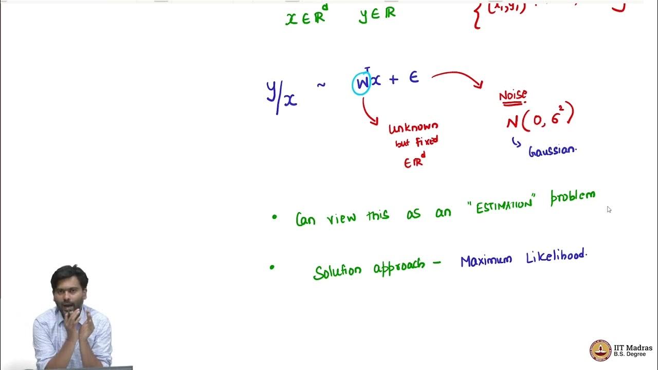
- 🧩 It explains the probabilistic viewpoint of linear regression, where y given x is a result of W transpose x plus Gaussian noise.
- 🔍 The script highlights that the W* from linear regression is the same as the maximum likelihood estimator for W, denoted as ŴML.
- 🤖 The maximum likelihood estimator ŴML is shown to be equivalent to assuming a squared error in the noise, which is a Gaussian assumption.
- 🔑 The script introduces the concept of using the estimator ŴML to understand its properties and gain insights into the problem.
- 📉 The importance of estimating the true W is emphasized, and the script discusses how to measure the 'goodness' of ŴML as an estimator.
- 📊 The script explains that ŴML is a random variable due to the randomness in y, and thus its estimation quality can vary.
- 📈 The concept of expected value is used to understand the average performance of ŴML in estimating W, considering the randomness in y.
- 📐 The script introduces the Euclidean norm squared as a measure to quantify the deviation between the estimated ŴML and the true W.
- 📘 It is mentioned that the average deviation of ŴML from the true W is proportional to the variance of the noise (sigma squared) and the trace of the inverse of the covariance matrix of the features.
- 🔄 The script suggests that while we cannot change the noise variance, we might be able to improve the estimator by considering the relationship between features.
Q & A
What is the problem of linear regression discussed in the script?
-The script discusses the problem of linear regression, focusing on deriving the optimal solution W* for the model and exploring the probabilistic viewpoint of linear regression where y given x is modeled as W transpose x plus noise.
What is the relationship between W* from linear regression and ŴML from maximum likelihood estimation?
-The script explains that W* derived from linear regression is exactly the same as ŴML, which is derived from the maximum likelihood estimation, given the assumption of Gaussian noise.
Why is it beneficial to view the linear regression problem from a probabilistic perspective?
-Viewing linear regression from a probabilistic perspective allows for the derivation of the maximum likelihood estimator for W, which provides insights into the properties of the estimator and helps in understanding the problem itself.
What does the script suggest about the properties of the maximum likelihood estimator ŴML?
-The script suggests that ŴML has nice properties that can provide insights into extending the linear regression problem, particularly in terms of how good it is as an estimator for the true W.
What is the significance of assuming Gaussian noise in the linear regression model?
-Assuming Gaussian noise is equivalent to assuming that the error is squared error, which simplifies the derivation of the maximum likelihood estimator and leads to the same solution as the optimal solution from linear regression.
How is the quality of the estimator ŴML measured in the script?
-The quality of ŴML is measured by looking at the expected value of the norm squared difference between ŴML and the true W, which is derived from considering the randomness in y.
What does the script imply about the randomness of y and its impact on ŴML?
-The script implies that since y is a random variable, ŴML, which is derived from y, is also random. This randomness affects the quality of ŴML as an estimator for the true W.
What is the expected value of the norm squared difference between ŴML and the true W?
-The expected value of the norm squared difference is given by sigma squared times the trace of the matrix (XX^T) pseudo-inverse or inverse, indicating the average deviation of ŴML from the true W.
How does the variance of the Gaussian noise (sigma squared) affect the quality of ŴML?
-The variance of the Gaussian noise directly affects the quality of ŴML, as a larger variance means more noise is added to W transpose X, leading to a larger average deviation between ŴML and the true W.
What role do the features in the data play in the quality of ŴML?
-The features in the data, represented by the trace of the matrix (XX^T) inverse, also affect the quality of ŴML. The relationship between the features influences the estimator's goodness.
Can the quality of ŴML be improved by manipulating the features in the data?
-The script suggests that while we cannot change the variance of the noise (sigma squared), we might be able to improve the quality of ŴML by manipulating the features in the data, although it does not specify how this can be achieved.
Outlines
📚 Introduction to Linear Regression and Estimation
This paragraph introduces the concepts of linear regression and the derivation of the optimal solution W*. It discusses the probabilistic perspective of linear regression, where y is expressed as W transpose x plus noise. The maximum likelihood estimator for w is derived, and it is shown that this estimator is equivalent to the solution obtained from linear regression. The paragraph also touches on the assumption of Gaussian noise and its implications on the error estimation, setting the stage for further exploration of the estimator's properties.
🔍 Evaluating the Estimator's Performance
The second paragraph delves into evaluating the performance of the maximum likelihood estimator (W hat ML) for W. It discusses the concept of measuring the estimator's accuracy by examining the norm squared difference between W hat ML and the true W. The importance of considering the average performance over multiple datasets due to the randomness of y is emphasized. The paragraph introduces the idea of calculating the expected value of this norm squared difference to understand the estimator's average deviation from the true W, highlighting the need for a deeper understanding of the estimator's properties.
📉 The Impact of Noise and Data Features on Estimation
This paragraph explores how the variance of the Gaussian noise (sigma squared) and the relationship between data features affect the estimator's performance. It explains that the average deviation of W hat ML from the true W is influenced by both the noise variance and the trace of the inverse of the covariance matrix of the features. The paragraph suggests that while the noise variance is a given factor, the structure of the features in the dataset could potentially be manipulated to improve the estimator's performance, although it acknowledges that this is a complex and uncertain proposition.
Mindmap
Keywords
💡Linear Regression
💡Probabilistic Viewpoint
💡Maximum Likelihood Estimation (MLE)
💡Gaussian Noise
💡Estimator
💡Euclidean Norm
💡Expected Value
💡Trace
💡Pseudoinverse
💡Covariance Matrix
💡Mean Squared Error (MSE)
Highlights
Derivation of the optimal solution W* for linear regression.
Introduction of a probabilistic viewpoint for linear regression.
Identification of y given x as W transpose x plus Gaussian noise.
Observation that W* from linear regression equals ŴML from maximum likelihood estimation.
Assumption of Gaussian noise leading to squared error assumption.
Discussion on the benefits of viewing ŴML as an estimator.
Understanding ŴML as an estimator for the true W in a probabilistic model.
Exploration of the properties of the estimator ŴML.
Importance of the Euclidean norm in measuring the goodness of ŴML.
Concept of expected value in assessing ŴML's performance.
The randomness of y affecting the estimator ŴML.
The impact of data variability on the estimator's quality.
The derivation of the expected value of the deviation between ŴML and the true W.
The expression of the average deviation in terms of sigma squared and the trace of XX^T.
The role of noise variance in the quality of the estimator.
The influence of feature relationships on the estimator's performance.
The potential for tweaking feature relationships to improve the estimator.
Transcripts
Hello.
So for, we have looked at the problem of linear regression, and we derive the optimal
solution W star for linear regression. And then we said that we can look at a
probabilistic viewpoint for linear regression. And we said that the y given x will be some W
transpose x plus 0 mean noise, and derive the maximum likelihood estimator for w. And we
observed that the w star that comes from linear regression is exactly same as w hat ML, which
comes from the maximum likelihood estimation. So, this comes from maximum likelihood.
So, which gave us the idea that, if we assume that the noise is Gaussian, then that is equivalent to
assuming that the error is squared error. So, then we ask the question, what else is the benefit of
viewing this as an estimator? That is W hat ML is an estimator for W and what other properties can
we look at of this estimator that will help us gain some insights about this problem itself.
And now, what we are going to look at is one nice property of this estimator which will
give us some insights into extending the linear regression problem in a particular direction.
For that, let us try to understand how good as an estimator W hat ML is.
Remember, there is some w such that y given x is W transpose X plus some epsilon,
where epsilon we said is, is a Gaussian noise with mean 0 and some variance sigma squared.
This is what our assumption was. So, which means that for every x in our data,
the y was generated using some w transpose x, some unknown but fixed w, which we do not know,
and then adding a 0 mean Gaussian noise, which means that the y given x itself can be thought of
as a Gaussian with mean w transpose x and sigma squared. This is what we have seen so far.
Now, our W hat ML is trying to estimate what is this W? It is a guess for this W. So,
now we can ask the question, how good is W hat ML as a guess for the true w. Now, how can we
measure this goodness, remember, W is some vector which is unknown, but is in some d dimension. So,
where d is the number of features. So, it is W hat ML, W hat ML is also
in d dimension, because it is an estimator for w. However, W hat ML
is derived out of an optimization problem. That is we maximize the likelihood and get W hat ML as
the solution of an optimization problem. And this optimization problem involves data, which involves
x and y. And we are assuming y is random. That is y has some random component. So,
the y is a random variable. So, if y is random, then the likelihood estimator,
the best estimator for w is also going to be random, because it depends on y.
So, if you are trying to see which w maximizes our chance of seeing all the y's y1, y2 tell yn
and so the w is going to be some function of the underlying y, and y because y is random. So, it is
W. So, now what could happen is that in if we try to understand W hat ML for some realization
of our data points, let us say you have some data x1 to xn, x1, y1 let us say till xn, yn.
Now of course, y is random x, we not assuming anything about x, y is random.
Now, it might be the case that the y's that we have got
are not in representative of the underlying W. In other words, we might have had a very extremely
unlucky day that these noise values when you are computing y's, so y1 is W transpose x1 plus some
noise epsilon 1, maybe this noise is too high. So, in our data that we get, and so this y's are
not really giving us enough information about W which means that if y’s are very noisy, then the w
that we are going to calculate is also going to be kind of bad. So, we cannot decide how good is our
W hat ML with respect to just a single data set. Instead, we can ask, well, because y’s are random
so is W hat ML, we can ask on an average. How does our random W hat ML, perform in estimating W.
So, one way to capture this is by looking at the following quantity, we can we want a way
to understand the goodness of W hat ML, how good W hat ML is in estimating W.
So, one way to understand this is to look at W hat ML minus w. And because these are d dimensional
vectors, you can look at their norm squared. So, when I say norm, it is like the Euclidean
norm, the distance between these two vectors. But now, again, because we cannot just look at
one sample, one data set and decide this, we want to understand this on an average,
how does this happen, which means we need to look at the expected value of this quantity.
What is the expected value? Well, the expected value is the average expectation
over the randomness in y that is, it is as if one way to think about this is that let
us say we create one data set where their y’s are derived random according to W transpose
x plus Gaussian 0 mean Gaussian noise. Now, you calculate the W hat ML for this
data set and see how far away W hat ML is with respect to W. Now, you do the same experiment
many-many times and then average the distance between W hat ML’s that you get with respect
to the true W, so the distance squared. Now, this average will slowly converge to
the expected value of this random variable. So, this is one way to think about what we are trying
to compute. So, on an average, where the average is over all possible data sets that you can get,
so, we are all possible randomness in y, what is the average deviation of W hat ML with respect
to the true W, we can try to ask this. So, this is a quantity of interest for us.
I will not really derive this quantity. Because I mean, it is not too hard to derive this, but let
us not go and derive this right now. Instead, I will tell you what this quantity is? So, actually,
it is not too hard to derive this because once you know what is the quantity, what is W hat ML as a
function of x and y, which we already know is just X transpose, X, X transpose we know that W
hat ML is just X X transpose pseudo inverse x y. So, this is something that we have already seen.
Now, y is the random part and you can use the properties of y and so on to derive what this
value is. But what I am going to do here is just to give you the value, those who are interested
can try and actually compute this value for yourself. It is a bit of not too much of an,
I mean just an algebraic derivation. So, what is this value? This value turns out to be
an interesting quantity, and we will see why it is interesting. I will first put down what this value
is? This value turns out to be sigma squared into the trace of XX transpose, pseudo inverse
or inverse. So, both are okay. So, this is telling us something very interesting.
The average deviation between your estimated W hat ML and W, the true W is a product of two terms.
One term is sigma squared, which is the variance of the noise that you add to W transpose X.
Now, this variance should somehow affect our quality of W hat ML. That is very clear. So,
because if I add noise, if I add more noise. Which means that if I add a 0 mean noise with the
larger variance, which means that I am confusing my W hat, W transpose X value with more noise. And
so my quality should go down. So, which means that the more the variance is, the more the average
deviation between W hat ML and true W would be, so, the sigma squared, remember sigma squared
is just the variance of the Gaussian noise. So, that we add to W transpose X. So, that should
directly affect our quality of our estimator which is fine, which is what is happening.
But what this interestingly tells us is that it not only depends on sigma squared,
it also depends on the data features themselves. So, it depends on the features via the trace of
the matrix X X transpose inverse which is like the inverse of your covariance matrix. So,
we can even for simplicity, we can just assume that this is an inverse that is still,
which means now it is not. So now, depending on how the
features themselves are related to each other will also affect our,
Estimators Goodness. So, it is not just the noise that y has with respect to, W transpose
X plus whatever noise you add, of course, that is going to affect but that is not the only thing.
It is also how the features are related to each other, which is an interesting thing to observe.
Well, there is some data generating process. So, we are given the data, and we are assuming
that is this data generating process, which is adding this Gaussian noise to our labels
and then giving us the y's. So, we cannot change this data generating process, which means that we
do not have any control over sigma squared as such. But then the features are given to us.
So, now the question is, we cannot really touch sigma squared, because it is some
noise that gets added and then it is given to us. But we are given X and then the features
themselves somehow affect the goodness of W hat ML. So, can we somehow tweak this or play
around with this to get a better estimator, which perhaps will have lesser mean squared error?
We do not know that is even possible. But if at all, it is possible, it is going to be,
you have to touch this term, because sigma squared is anyway out of question,
because that is a noise that is in some sense, you have to suffer that much. Can we somehow get rid,
I mean, not get rid of can you somehow at least reduce this part or at least focus on this part
is the next valid question that we can ask. And let us see what we can do with this.
浏览更多相关视频
Probabilistic view of linear regression
Relation between solution of linear regression and ridge regression
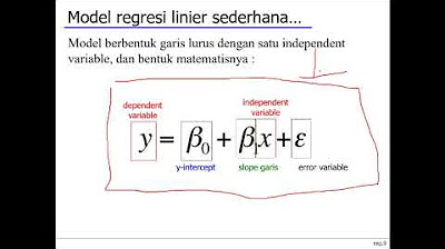
Ridge regression
Linear Regression, Cost Function and Gradient Descent Algorithm..Clearly Explained !!
Week 2 Lecture 6 - Statistical Decision Theory - Classification
36. Regressione: bontà d'adattamento
5.0 / 5 (0 votes)