Probabilistic view of linear regression
Summary
TLDRThis video script explores the probabilistic perspective of linear regression, treating it as an estimation problem. It explains how the labels are generated through a probabilistic model involving feature vectors, weights, and Gaussian noise. The script delves into the maximum likelihood approach to estimate the weights, leading to the same solution as linear regression with squared error. It emphasizes the equivalence between choosing a noise distribution and an error function, highlighting the importance of Gaussian noise in justifying the squared error commonly used in regression analysis.
Takeaways
- š The script introduces a probabilistic perspective on linear regression, suggesting that labels are generated through a probabilistic model involving data points and noise.
- š It explains that in linear regression, we are not modeling the generation of features themselves but the probabilistic relationship between features and labels.
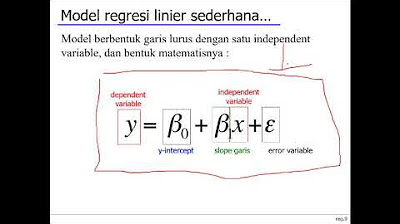
- šÆ The model assumes that each label y_i is generated as w^T x_i + epsilon, where epsilon is noise, and w is an unknown fixed parameter vector.
- š The noise epsilon is assumed to follow a Gaussian distribution with a mean of 0 and a known variance sigma^2.
- š§© The script connects the concept of maximum likelihood estimation to the problem of linear regression, highlighting that the maximum likelihood approach leads to the same solution as minimizing squared error.
- š The likelihood function is constructed based on the assumption of independent and identically distributed (i.i.d.) data points, each following a Gaussian distribution influenced by the model's parameters.
- āļø The log-likelihood is used for simplification, turning the product of probabilities into a sum, which is easier to maximize.
- š§ By maximizing the log-likelihood, the script demonstrates that the solution for w is equivalent to the solution obtained from traditional linear regression with squared error loss.
- š The conclusion emphasizes that the maximum likelihood estimator with 0 mean Gaussian noise is the same as the solution from linear regression with squared error, highlighting the importance of the noise assumption.
- š The script points out that the choice of error function in regression is implicitly tied to the assumed noise distribution, and different noise assumptions would lead to different loss functions.
- š Viewing linear regression from a probabilistic viewpoint allows for the application of statistical estimator theory to understand and analyze the properties of the estimator, such as hat{w}_{ML}.
- š” The script suggests that by adopting a probabilistic approach, we gain insights into the properties of the estimator and the connection between noise statistics and the choice of loss function in regression.
Q & A
What is the main focus of the script provided?
-The script focuses on explaining the probabilistic view of linear regression, where the relationship between features and labels is modeled probabilistically with the assumption of a Gaussian noise model.
What is the probabilistic model assumed for the labels in this context?
-The labels are assumed to be generated as the result of the dot product of the weight vector 'w' and the feature vector 'x', plus some Gaussian noise 'Īµ' with a mean of 0 and known variance ĻĀ².
Why is the probabilistic model not concerned with how the features themselves are generated?
-The model is only concerned with the relationship between features and labels, not the generation of the features themselves, as it is focused on estimating the unknown parameters 'w' that affect the labels.
What is the significance of the noise term 'Īµ' in the model?
-The noise term 'Īµ' represents the random error or deviation in the label 'y' from the true linear relationship 'w transpose x', and it is assumed to follow a Gaussian distribution with 0 mean and variance ĻĀ².
How does the assumption of Gaussian noise relate to the choice of squared error in linear regression?
-The assumption of Gaussian noise with 0 mean justifies the use of squared error as the loss function in linear regression, as it implies that the likelihood of observing a label 'y' given 'x' is maximized when the squared error is minimized.
What is the maximum likelihood approach used for in this script?
-The maximum likelihood approach is used to estimate the parameter 'w' by finding the value that maximizes the likelihood of observing the given dataset, under the assumption of the probabilistic model described.
What is the form of the likelihood function used in the script?
-The likelihood function is the product of the Gaussian probability densities for each data point, with each density having a mean of 'w transpose xi' and variance ĻĀ².
Why is the log likelihood used instead of the likelihood function itself?
-The log likelihood is used because it simplifies the optimization process by converting the product of likelihoods into a sum, which is easier to maximize.
What is the solution to the maximization of the log likelihood?
-The solution is to minimize the sum of squared differences between the predicted labels 'w transpose xi' and the actual labels 'yi', which is the same as the solution to the linear regression problem with squared error.
How does the script connect the choice of noise distribution to the loss function used in regression?
-The script explains that the choice of noise distribution (e.g., Gaussian) implicitly defines the loss function (e.g., squared error), and vice versa, because the loss function reflects the assumed statistical properties of the noise.
What additional insights does the probabilistic viewpoint provide beyond the traditional linear regression approach?
-The probabilistic viewpoint allows for the study of the properties of the estimator 'w hat ML', such as its statistical properties and robustness, which can lead to a deeper understanding of the regression problem.
Outlines
š Probabilistic View of Linear Regression
This paragraph introduces the concept of viewing linear regression through a probabilistic lens, where labels are generated by a probabilistic model rather than a deterministic one. It explains that the model assumes labels are produced as the result of a linear combination of features plus some noise (epsilon), which is assumed to be Gaussian with a mean of zero and a known variance (sigma squared). The focus is on estimating the unknown parameter 'w', which represents the relationship between features and labels. The paragraph also outlines the maximum likelihood approach as a method to estimate 'w', setting the stage for further exploration into the probabilistic underpinnings of linear regression.
š Maximum Likelihood Estimation in Linear Regression
The second paragraph delves into the specifics of using the maximum likelihood estimation (MLE) to solve the linear regression problem. It discusses the likelihood function, which is based on the assumption of independent and identically distributed (i.i.d.) Gaussian noise with zero mean and a known variance. The paragraph explains how the likelihood function is constructed and how taking the logarithm of the likelihood simplifies the maximization process. It also highlights that maximizing the likelihood is equivalent to minimizing the sum of squared differences between the predicted and actual labels, a problem already familiar from standard linear regression. The solution to this minimization problem is identified as the MLE estimator, which is the same as the solution obtained from the least squares method in linear regression.
š Equivalence of MLE and Squared Error in Linear Regression
The final paragraph emphasizes the equivalence between the maximum likelihood estimator assuming zero-mean Gaussian noise and the solution to the linear regression problem with squared error. It points out that choosing squared error as the loss function implicitly assumes Gaussian noise in the model. The paragraph also discusses the implications of this connection, noting that if the noise were not Gaussian, the solutions to the MLE and squared error problems would no longer be equivalent, and a different loss function would be appropriate. Additionally, it suggests that viewing the problem probabilistically allows for a deeper understanding of the estimator's properties and introduces the idea that further exploration into the properties of the MLE estimator will be conducted.
Mindmap
Keywords
š”Probabilistic View
š”Linear Regression
š”Estimation Problem
š”Data Points
š”Labels
š”Noise
š”Gaussian Distribution
š”Maximum Likelihood
š”Log Likelihood
š”Error Function
š”Pseudo Inverse
Highlights
Introduction to a probabilistic view of linear regression, treating it as a probabilistic model for generating labels.
Assumption of a probabilistic mechanism that generates labels based on data points and noise.
Discussion on the probabilistic model where labels are generated as the sum of a feature's dot product with weights and noise.
Clarification that the model does not attempt to model the generation of features themselves.
Introduction of noise as a Gaussian distribution with a mean of zero and known variance.
Explanation of the dataset generation process involving an unknown but fixed parameter w.
The problem is framed as an estimation problem where the goal is to estimate the weights w.
Introduction of the maximum likelihood approach as a method to estimate the weights.
Formulation of the likelihood function for the linear regression model with Gaussian noise.
Log-likelihood is used for ease of computation in the maximization process.
The maximization of the log-likelihood leads to the minimization of the squared error, a familiar problem in linear regression.
Derivation of the maximum likelihood estimator for linear regression, which matches the solution from the squared error approach.
Equivalence of the maximum likelihood estimator with squared error in linear regression under the assumption of Gaussian noise.
Implication that the choice of squared error in linear regression implicitly assumes Gaussian noise.
Discussion on the impact of noise statistics on the choice of loss function in regression models.
Exploration of alternative noise distributions and their corresponding loss functions, such as Laplacian noise leading to absolute error.
Advantage of the probabilistic viewpoint for studying the properties of estimators in linear regression.
Transcripts
ļ»æ Ā
Now, what we are going to see is aĀ probabilistic view of linear regression.Ā Ā
What happens when you think of linear regressionĀ as if there is some probabilistic model thatĀ Ā
generates our labels. So, that is what, thatĀ is what we are going to look at. So, we haveĀ Ā
already looked at estimation, in general in anĀ unsupervised setting where we have seen maximumĀ Ā
likelihood Bayesian methods and so on. But now, weĀ are going to think of our linear regression alsoĀ Ā
as in some sense an estimation problem, whichĀ means that there should be some probabilisticĀ Ā
mechanism that we are going to assume thatĀ generates something that we have seen. Ā
So, what is that we are going to assume?Ā Well, in the linear regression problem,Ā Ā
you have the data points in d dimension, theĀ labels are in real numbers and of course,Ā Ā
you have a dataset which I can write as x1Ā y1 dot dot dot xn yn this is the dataset.Ā Ā
Now, the probabilistic model that we are goingĀ to assume is as follows, we are going to assumeĀ Ā
that the label is generated as follows theĀ label given the data point is generated asĀ Ā
w transpose x plus some noise epsilon. What does this mean? This means thatĀ Ā
I do not I am not trying to model how theĀ features themselves are generated, I am justĀ Ā
trying to model the relationship between featuresĀ and the labels in a probabilistic way, and what isĀ Ā
the probabilistic mechanism that generates theĀ labels if I give you x, well, what we are goingĀ Ā
to posit or hypothesize is the following. So, if I give you a feature, then there is anĀ Ā
unknown but fixed w which is not known to us,Ā so, this is the parameter of the problem. So,Ā Ā
this is unknown, but fixed and this is an Rd andĀ whenever a feature is seen you do a w transpose x,Ā Ā
but then your y is not exactly w transpose x.Ā So, this is the structure part of the problem. Ā
Now, we are going to explicitly say thereĀ is also a noise part to the problem. So,Ā Ā
we are adding some noise to this w transpose xĀ and that is this epsilon. So, this epsilon isĀ Ā
noise and this noise is we are going to assumeĀ is a Gaussian distribution with 0 mean and someĀ Ā
known variance sigma squared. So, this is Gaussian, Gaussian.Ā Ā
So, so, now, what we are saying is that ourĀ data set every yi was generated according toĀ Ā
this process somebody was gave us xi and thenĀ to get the yi there is an unknown but fixed wĀ Ā
using which w transpose xi was generated and thenĀ a noise got added and we are only seeing the noisyĀ Ā
version of w transpose xi whereas we know that theĀ statistics of this noise is 0 mean and some (va)Ā Ā
known variance sigma squared, all that is known. So, but the only thing that is unknown for us is wĀ Ā
we do not know w so, which meansĀ now, we can view the whole thingĀ Ā
as an estimation problem. So, now we can view we can view thisĀ Ā
as an estimation problem, what are we trying toĀ estimate? Well, we are trying to estimate the wĀ Ā
which after adding noise affects our labels.Ā So, once we have put down a model as to howĀ Ā
the data is generated, at least the y is given xĀ is generated, and we have an unknown parameter. Ā
Now, we already know what some methodsĀ to estimate come up with estimatorsĀ Ā
and the simplest method that we have alreadyĀ seen. The solution approach to this problemĀ Ā
is, as you must have already guessed,Ā is just the maximum likelihood approach.Ā Ā
So, now I want to understand the same problem,Ā but then in a maximum likelihood context andĀ Ā
see what comes out of it. So, which means the standard maximumĀ Ā
likelihood problem, I am going toĀ write the likelihood, so the likelihoodĀ Ā
function is going to look like this. Let us callĀ this x. Now, what is the parameter of interest,Ā Ā
well the parameter of interest is W, but then theĀ likelihood function also depends on the data x1Ā Ā
to xn and y1 to yn, because this is the observedĀ data points, we are observing this and then weĀ Ā
are treating this as if it is a function of W. Though, it is also a function of the data pointsĀ Ā
and the labels, but then we are going toĀ treat it as a function of w and then weĀ Ā
will try to find that w that maximizesĀ our likelihood of seeing this, but thenĀ Ā
before that, what is this likelihood itself. Now, as usual, the i.i.d. assumptions hold in aĀ Ā
probabilistic model that is x1 y1 is independentlyĀ generated. So, y1 is independently generated of y2Ā Ā
and so on and they are all from the same GaussianĀ distribution. So, basically, this is going toĀ Ā
be product of i equals 1 to n. Now, what is theĀ chance that I see a particular yi for a given xi?Ā Ā
Well, we know that every yi given xi isĀ generated according to w transpose xi,Ā Ā
which is a fixed quantity, there is nothingĀ random there and then you add a random noise. Ā
But this noise is 0 mean noise with a certainĀ variance. So, if I add a constant fixed quantityĀ Ā
w transpose X site to the 0 mean Gaussian,Ā just the mean gets shifted, the variance spreadĀ Ā
is is fixed, but just the mean moves around byĀ adding a constant, let us say we have a 0 meanĀ Ā
Gaussian, I add 5 to it, it becomes a GaussianĀ with mean 5, the variance is still the same. So,Ā Ā
it is exactly the same thing here. Now, I have added w transpose xi to thisĀ Ā
0 mean Gaussian for the ith data point. So, now,Ā that would be a Gaussian distribution with meanĀ Ā
w transpose xi and variance sigma squared,Ā which we are assuming is known. Ā
So, now this would then be the likelihoodĀ can be written as the density of e,Ā Ā
which looks like e power, w transpose xi,Ā which is the mean, minus what I observed,Ā Ā
which is yi squared by 2 sigma squared andĀ of course, with 1 by square root 2 pi sigma.Ā Ā
Though let us content it does not really matterĀ in our in our maximization as we will see. Ā
So, once we have put down this likelihood,Ā I can now do the log likelihood log L of W,Ā Ā
with respect to the same parameters, x1 to xn y1Ā to yn. We want to do the logarithm because it isĀ Ā
hard to deal with products, easier to deal withĀ sums. So, this is sum over i equals one to n, theĀ Ā
log cancels the exponential. So, this is minus, wĀ transpose xi minus yi squared by 2 sigma squaredĀ Ā
to 1 by square root 2 pi sigma. Now, remember,Ā we want to think of this as a function of W.Ā Ā
x is our constant, sigma is our constant,Ā everything else, y is our constant,Ā Ā
so it is only a function of W. And we want to see which w maximizes ourĀ Ā
likelihood or log likelihood, whichĀ means I can equivalently equivalentlyĀ Ā
w star, I mean, to get the best w. I could haveĀ maximized. So, the mean, I want to maximize overĀ Ā
W, sum over i equals 1 to n, I am going toĀ remove, I do not care about these variables,Ā Ā
these are just constant scalings, these areĀ known sigma squared is assumed to be known. So,Ā Ā
these are constants, I do not care aboutĀ them. I will just hold on to the other guys. Ā
So, this is just w transpose xi minus yiĀ squared, of course, the minus is there. Now,Ā Ā
this is equivalent to minimizing over w sum overĀ i equals 1 to n w transpose xi minus yi squared.Ā Ā
Now, this minimization problem is somethingĀ that we have already encountered. So,Ā Ā
this is exactly the linear regression problemĀ with squared error that we already put out,Ā Ā
which means we know theĀ solution to this. Ā
So, so basically, what is the solution toĀ this? Well, then, the w hat ML as an estimatorĀ Ā
is exactly same as our w star, which we alreadyĀ know is x x transpose pseudo inverse x yĀ Ā
from our previous discussionĀ about linear regression.Ā Ā
Now, it is great that we started with a completelyĀ different technique of looking at things which isĀ Ā
by thinking of a probabilistic mechanism forĀ generating y given x and then did the mostĀ Ā
natural thing which is to look at a maximumĀ likelihood approach and outcomes solution,Ā Ā
which is exactly same as theĀ linear regression solution. Ā
So, what is the conclusion and it meritsĀ separate writing here because in someĀ Ā
interesting points can be made theĀ conclusion is that maximum likelihoodĀ Ā
estimator assuming this is the mostĀ important part 0 mean, Gaussian noiseĀ Ā
is exactly same as linear regressionĀ Ā
with and again, this is theĀ important part with squared error. Ā
We could have either solved the linear regressionĀ part with squared error, or we could have treatedĀ Ā
this problem as a maximum likelihood problem withĀ Gaussian noise with 0 mean Gaussian noise andĀ Ā
these both are exactly equivalent. These both areĀ equivalent is is an important thing to understand,Ā Ā
because what exactly makes them equivalent isĀ the choice of squared error when we startedĀ Ā
by looking at linear regression where we didĀ not really justify a squared error that much,Ā Ā
we just said that, well, we will start withĀ squared error because it looks like an intuitiveĀ Ā
thing to do do do, I mean, look at. Now, we are saying, well, more thanĀ Ā
just intuition, it has a very wellĀ probabilistic backing as well. So,Ā Ā
we are saying that if we chose squared errorĀ to solve the linear regression problem, it isĀ Ā
as if we are implicitly making the assumptionĀ that there is a Gaussian noise 0 mean that getsĀ Ā
added to our labels that corrupts our labels. Now, these two are both important to understand.Ā Ā
So, if I had changed my noise, if there isĀ reason to believe that my noise was not Gaussian,Ā Ā
then it would not be the same as solving theĀ linear regression problem is squared error. Ā
So, the noise statistics are the density that youĀ are assuming about the noise impacts, essentially,Ā Ā
the loss function, or the error function that weĀ are using in our linear regression. That is theĀ Ā
connection that I want you to make here. So, for example, if I hadĀ Ā
given a different noise, for instance, if there ifĀ I tried a different noise, like laplacian noise orĀ Ā
something like that, so I am just giving you anĀ example, then no longer you would end up withĀ Ā
a linear regression with squared error, theseĀ two will not be equivalent anymore, it wouldĀ Ā
be equivalent to a different loss function. Let us say in fact, and if if I mean just forĀ Ā
completions sake, if you use a laplacianĀ noise, then it would be as if you are,Ā Ā
you are looking at the absolute differenceĀ between w transpose xi and yi and then summingĀ Ā
up over them and that would be the problemĀ that you are actually trying to solve. Ā
So, because the laplacian PDF has an absoluteĀ value sitting at the top of exponential e powerĀ Ā
minus absolute value of w transpose xi minusĀ yi, it it it kind of falls down sharper thanĀ Ā
the Gaussian distribution but that that isĀ not the important point. The important pointĀ Ā
is that choosing a noise means implicitlyĀ choosing an error function and vice versa,Ā Ā
choosing an error function means implicitlyĀ choosing a noise, so that is the first connectionĀ Ā
that we want to make, which is which is importantĀ so, good so, we have made that connection. Ā
The question is, is this the only thingĀ that we gain, or are we gaining anythingĀ Ā
else by looking at this from a probabilisticĀ viewpoint, well, the answer is yes, this is anĀ Ā
important conclusion that we are drawing thatĀ if you view your w as an estimator, then youĀ Ā
can connect the noise and the loss. But now what else have we gained? So, what else,Ā Ā
what else have we gained,Ā Ā
by viewing this in a probabilistic way,Ā well, the most important thing that weĀ Ā
might have (perf) perhaps gainedĀ is that now we can study propertiesĀ Ā
of estimator especially to w hat ML.Ā Ā
So, this is an important gain that we have whenĀ we view learning as a probabilistic mechanism,Ā Ā
because the moment you put probabilistic learningĀ becomes estimation and once you have an estimator,Ā Ā
then you can bring in all the machinery thatĀ we know about understanding estimators. WeĀ Ā
have already seen some kind of understanding whatĀ are good estimators and whatever perhaps not. Ā
So, now, what we are going to see is can weĀ somehow use this notion of estimators that somehowĀ Ā
can we use some properties of these estimatorsĀ or some other way of trying to do estimation toĀ Ā
understand this problem of linear regressionĀ better and that is what we will do next.
Browse More Related Video
Goodness of Maximum Likelihood Estimator for linear regression
äøå¤ćēµ±čØåøļ¼čæ“ęøåę
What are Maximum Likelihood (ML) and Maximum a posteriori (MAP)? ("Best explanation on YouTube")
Regression and R-Squared (2.2)
Linear Regression, Cost Function and Gradient Descent Algorithm..Clearly Explained !!
Ridge regression
5.0 / 5 (0 votes)