[CS 70] Markov Chains – Finding Stationary Distributions
Summary
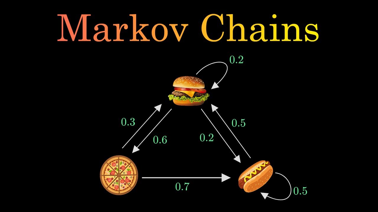
TLDRThe video script explains the concept of a stationary or invariant distribution in a Markov chain. It demonstrates how to find such a distribution by solving a system of linear equations where the multiplication of the transition matrix and the row vector of probabilities yields the same distribution. The example involves a simple Markov chain with two states, A and B, with given transition probabilities. The solution involves simplifying the equations and using the property that the probabilities must sum to 1, leading to the stationary distribution vector (4/11, 7/11).
Takeaways
- 📚 Pi sub n is the probability distribution at time step n, calculated as Pi sub 0 times P to the power of n.
- 🔄 The row vector Pi changes at each time step in a Markov chain, but there is a special case where it remains constant.
- 🌟 A stationary or invariant distribution is when multiplying the transition matrix P with Pi results in the same Pi.
- 🧩 To find a stationary distribution, solve the system of linear equations Pi P = Pi.
- 🔍 An example Markov chain is provided with two states A and B, with specific transition probabilities.
- 📉 The transition matrix is a 2x2 matrix, and rows must sum to 1 for the matrix to be correct.
- 🔢 The equations derived from Pi P = Pi are 0.3 Pi A + 0.4 Pi B = Pi A and 0.7 Pi A + 0.6 Pi B = Pi B.
- 🔄 Simplifying the equations leads to redundant equations, indicating a need for additional constraints.
- 🔄 The sum of elements in Pi must equal 1, which provides the necessary second equation to solve for Pi A and Pi B.
- 🔑 The solution to the equations is Pi A = 4/11 and Pi B = 7/11, forming the stationary distribution for the given Markov chain.
Q & A
What is a stationary distribution in the context of a Markov chain?
-A stationary distribution, also known as an invariant distribution, is a probability distribution that remains unchanged when multiplied by the transition matrix of a Markov chain. This means that if you apply the transition probabilities to the distribution, you get the same distribution back.
How do you determine if a distribution is stationary in a Markov chain?
-To determine if a distribution is stationary, you solve the system of linear equations where the product of the transition matrix and the distribution vector equals the distribution vector itself. If such a solution exists, the distribution is stationary.
What is the condition for the rows of a transition matrix to be valid?
-The rows of a transition matrix must sum to 1. This ensures that the probabilities of transitioning from one state to all possible states add up to the certainty of a transition occurring.
What is the significance of the transition matrix in a Markov chain?
-The transition matrix in a Markov chain represents the probabilities of moving from one state to another in the chain. Each element in the matrix corresponds to the probability of transitioning from one specific state to another.
How many states does the Markov chain in the example have?
-The Markov chain in the example has two states, labeled as 'a' and 'b'.
What are the probabilities of transitioning from state 'a' to state 'b' and vice versa in the given example?
-In the example, the probability of transitioning from state 'a' to state 'b' is 0.7, and the probability of transitioning from state 'b' to state 'a' is 0.4.
What is the self-loop probability for state 'a' in the example Markov chain?
-The self-loop probability for state 'a', which is the probability of staying in state 'a', is 0.3.
What is the self-loop probability for state 'b' in the example Markov chain?
-The self-loop probability for state 'b', which is the probability of staying in state 'b', is 0.6.
Why can't the system of equations be solved directly in the example provided?
-The system of equations in the example is redundant, meaning that the equations do not provide enough independent information to solve for both unknowns (PI_a and PI_b). This redundancy occurs because the equations essentially state the same relationship.
How is the second equation used to solve for the stationary distribution in the example?
-The second equation is derived from the requirement that the elements of the probability distribution must sum to 1. This non-redundant equation, combined with the relationship between PI_a and PI_b, allows for the calculation of the stationary distribution.
What is the final stationary distribution for the Markov chain in the example?
-The final stationary distribution for the Markov chain in the example is a row vector with elements 4/11 and 7/11, representing the probabilities of being in states 'a' and 'b', respectively.
Outlines
🧩 Introduction to Stationary Distributions in Markov Chains
This paragraph introduces the concept of a stationary distribution in the context of Markov chains. It explains that the row vector \( \pi \), representing the probability distribution, changes at each time step when multiplied by the transition matrix \( P \). However, there is a special case where the multiplication of \( \pi \) and \( P \) results in the same distribution, making \( \pi \) a stationary or invariant distribution. The method to find such a distribution involves solving the system of linear equations \( \pi P = \pi \). The paragraph also sets the stage for an example involving a Markov chain with two states, A and B, and their respective transition probabilities.
🔍 Solving for the Stationary Distribution in a Two-State Markov Chain
This paragraph delves into the process of finding a stationary distribution for a specific two-state Markov chain with states A and B. The transition probabilities are given, and the transition matrix is constructed accordingly. The rows of the matrix are checked to ensure they sum to 1, which is a necessary condition for a valid transition matrix. The equation \( \pi P = \pi \) is then used to set up a system of equations to solve for the probabilities \( \pi_A \) and \( \pi_B \). Initially, the equations appear redundant, but by recognizing that the elements of \( \pi \) must sum to 1, a second equation is derived. This leads to the solution where \( \pi_A = \frac{4}{11} \) and \( \pi_B = \frac{7}{11} \), thus identifying the stationary distribution for the given Markov chain.
Mindmap
Keywords
💡pi sub n
💡transition matrix
💡stationary distribution
💡invariant distribution
💡linear equations
💡Markov chain
💡probability distribution
💡self-loop
💡sanity check
💡redundant equations
💡row vector
Highlights
Pi sub n is defined as the product of pi sub 0 and P to the power of n, representing the evolution of a probability distribution over time in a Markov chain.
A row vector PI is expected to change at each time step in a Markov chain due to the multiplication by the transition matrix P.
A stationary or invariant distribution is a special case where the multiplication of PI by the transition matrix P yields the same probability distribution.
To find a stationary distribution, one must solve the system of linear equations PI P equals PI.
An example Markov chain with states A and B is introduced, with specific transition probabilities between them.
The transition matrix for the example Markov chain is a 2x2 matrix with probabilities summing to 1 for each row.
The sanity check for the transition matrix involves ensuring that the sum of probabilities in each row equals 1.
The solution for the stationary distribution involves setting up and solving the equation PI P equals PI for the row vector PI.
The multiplication of the row vector PI by the transition matrix results in two equations that need to be solved.
Simplifying the equations by multiplying by ten makes the calculations more manageable.
The resulting equations after simplification are redundant, indicating that there is only one useful equation for solving the system.
The elements of the stationary distribution must sum to 1, providing a second non-redundant equation to solve the system.
The solution to the stationary distribution is found by using the relationship between PI(A) and PI(B) and the sum-to-one constraint.
The final stationary distribution for the example Markov chain is a row vector with probabilities 4/11 for state A and 7/11 for state B.
The process of finding a stationary distribution involves understanding the properties of Markov chains and applying linear algebra techniques.
The example demonstrates the practical application of finding a stationary distribution in a simple two-state Markov chain scenario.
The concept of a stationary distribution is crucial for understanding long-term behavior in stochastic processes modeled by Markov chains.
Transcripts
so as we've seen earlier pi sub n is
going to be equal pi sub 0 times P to
the N so in general you expect at each
time step your row vector PI to be
constantly changing however there is a
special case when the row vector pi when
multiplied this P does not change so
there's a special case where this
equation is satisfied pi times p is
equal to pi so when I multiply by my
transition matrix I get my same
probability distribution back and if
this is the case then we call pi a
stationary distribution or in other
words we call it an invariant
distribution and to find such a
distribution we typically just solve
this system of linear equations PI P is
equal to PI so now let's go over an
example of how to find a stationary
distribution in a Markov chain so
suppose I have the following Markov
chain with two states a and B a goes to
B with probability point seven B goes to
a with probability point four a self
loops with probability point three and B
has a self-loop with probability point
six so let's write out the probability
transition matrix here so it's a two by
two matrix since we have two states so a
goes to a with the probability point
three a goes to B with probability point
seven
B goes to a with probability 0.4 and
then B goes to B with probability 0.6
and just a quick sanity check to make
sure that your transition matrix is
correct is to check that the rows sum to
1 so in this case point 3 plus 0.7 is 1
and point 4 plus point 6 is also 1 and
then let's set our PI to be equal to the
row vector PI a and PI B so this is what
we're going to solve for and now let's
try to solve the equation PI P is equal
to PI so so if I multiply this row
vector by this matrix so I'm going to
get two equations the first equation is
going to be zero point three PI a plus
zero point four PI B is equal to PI a
and then the next equation I'm going to
get so I multiply this row vector by the
second column and I get zero point seven
PI a plus zero point six PI B is equal
to PI B so I'm going to multiply both of
these equations by ten just to make
everything easier to work with so I'm
going to have three PI a plus four PI B
is equal to 10 PI a and then seven PI a
plus 6 PI B is equal to 10 PI D so I'm
going to move this PI a to the other
side so this equation so this equation
I'm going to move the three PI a over to
the other side to get 4 PI B is equal to
7 PI and then I'm going to do the same
for this equation I'm going to move the
6 PI B over to the right side so I'm
going to get 7
a is equal to 4 PI B so now if you
notice these two equations are exactly
the same equation there are redundant
equations so as of right now we can't
actually solve this system of linear
equations because we have two unknowns
PI and PI B but we only have one useful
equation so what do we do well so I'm
going to let's see I'm gonna erase this
Markov chain so I have more room to work
with so what do we know about elements
in PI well we know that it's a valid
probability distribution so its elements
must sum to 1 and this is the equation
that we can use as our second
non-redundant equation so so I
previously have 4 pi B is equal to 7 PI
a so PI B is equal to 7 over 4 PI of a
and I'm going to plug this into this
equation to get PI of a plus 7 over 4 PI
of a is equal to 1 so 11 over 4 PI of a
is equal to 1 PI of a is equal to 4 over
11 and therefore PI of B is equal to 1
minus PI of a which is equal to 7 over
11 so therefore if I go over here so our
stationary distribution pi is just equal
to the row vector 4 / 11 sin 7 over 11
浏览更多相关视频
Markov Chains Clearly Explained! Part - 1
Introdução - Cadeias de Markov (Markov Chains) - Outspoken Market
Markov Decision Process (MDP) - 5 Minutes with Cyrill
Normal Distribution: Calculating Probabilities/Areas (z-table)
Poisson Distribution EXPLAINED in UNDER 15 MINUTES!
Markov Models | Markov Chains | Markov Property | Applications | Part 1
5.0 / 5 (0 votes)