HighScore Plus Tutorial - Phase Identification X-ray Diffraction - Long Version - JIAM Diffraction
Summary
TLDRIn this instructional video, Michael Koehler, lab manager at the JIAM Diffraction Facility, demonstrates how to utilize HighScore Plus software for phase identification in a sample. He guides viewers through loading data, background determination, peak marking, and refining the search for matching diffraction patterns. The tutorial emphasizes optimizing parameters for background adjustment, manually correcting peak identification errors, and narrowing down potential matches using chemical composition filters. The goal is to accurately match sample peaks with known diffraction patterns, concluding with phase identification.
Takeaways
- 📚 Michael Koehler introduces himself as the lab manager for the JIAM Diffraction Facility at the University of Tennessee, Knoxville.
- 📹 The video is a tutorial on using HighScore Plus software for phase identification in samples.
- 🔍 HighScore Plus supports various file types for data analysis, including XRDML, which was used in the demonstration.
- 🛠 The first step in phase identification is to load a data file and determine the background of the data, which can be done automatically or manually.
- 📉 The background determination involves adjusting parameters like 'bending factor' and 'granularity' to accurately represent the data's baseline.
- 🔍 'Search Peaks' is a feature that helps identify and differentiate peaks from background noise, refining the data for better analysis.
- 👀 It's important to review and correct the peak list generated by the software to ensure accuracy in phase identification.
- 📊 The 'Default Profile Fit' function helps improve the fit between the calculated pattern and the actual data, enhancing peak accuracy.
- 🔎 'Search Match' is used to find possible matches for the identified peaks against a database of patterns, with the results sorted by a scoring system.
- ⚙️ Refining search parameters, such as subfiles, chemistry, and crystallography, can significantly reduce the number of patterns to search through, speeding up the process.
- 🗂 The final step is to match the peaks to the correct phases by evaluating the candidate list and ensuring that all peaks have corresponding matches in the selected patterns.
Q & A
Who is the speaker in the video and what is his role?
-The speaker is Michael Koehler, and he is the lab manager for the JIAM Diffraction Facility at the University of Tennessee, Knoxville.
What is the purpose of the video?
-The video's purpose is to demonstrate how to use HighScore Plus software for phase identification in a sample.
What is the first step in phase identification using HighScore Plus according to the video?
-The first step in phase identification is to load a data file into HighScore Plus.
What file types are compatible with HighScore Plus?
-HighScore Plus can accommodate different types of files, including XRDML files, which are used when data is collected using a Panalytical instrument.
How does one determine the background in HighScore Plus?
-The background can be determined in HighScore Plus by going to 'Treatment' and selecting 'Determine Background.' Options include 'Automatic,' 'Manual,' and 'By Search Peaks.'
What is the significance of the 'Bending Factor' and 'Granularity' in determining the background?
-The 'Bending Factor' determines how much the background curve bends up into the peak, while 'Granularity' changes the distance between points of inflection in the background curve, affecting its ability to bend.
Why might one choose not to subtract the background in HighScore Plus?
-Subtracting the background can lead to negative intensity values, which Rietveld refinement does not handle well, and it may also obscure certain data points that are important for analysis.
What is the purpose of the 'Search Peaks' function in HighScore Plus?
-The 'Search Peaks' function helps identify and distinguish peaks from noise in the data, allowing the software to better understand and analyze the sample's diffraction pattern.
How can the 'Search Match' feature in HighScore Plus assist in phase identification?
-The 'Search Match' feature compares the identified peaks with a database of patterns to find potential matches, which can then be evaluated to determine the phases present in the sample.
What is the importance of refining search parameters in the 'Search Match' process?
-Refining search parameters helps to narrow down the number of patterns that need to be searched through, making the matching process more efficient and targeted to the specific characteristics of the sample.
How does the 'Chemistry' tab in HighScore Plus help in narrowing down potential matches?
-The 'Chemistry' tab allows the user to specify the elements believed to be present in the material and to ignore patterns that do not contain these elements, significantly reducing the number of potential matches.
What does the 'Score' column in the 'Search Match' results represent?
-The 'Score' column represents the probability of a match between the pattern and the sample's peaks, with higher scores indicating a better match, although it does not guarantee the presence of the phase in the sample.
How can one verify if a potential match from the 'Search Match' is accurate?
-Verification is done by clicking on the potential match and observing if the peaks in the diffraction pattern align with the peaks in the sample's data curve.
Outlines

此内容仅限付费用户访问。 请升级后访问。
立即升级Mindmap

此内容仅限付费用户访问。 请升级后访问。
立即升级Keywords

此内容仅限付费用户访问。 请升级后访问。
立即升级Highlights

此内容仅限付费用户访问。 请升级后访问。
立即升级Transcripts

此内容仅限付费用户访问。 请升级后访问。
立即升级浏览更多相关视频

Spektrofotometer UV Visible : Penentuan Panjang Gelombang Maksimum - STFI Edukasi
Performing Thin-Layer Chromatography to analyze organic samples
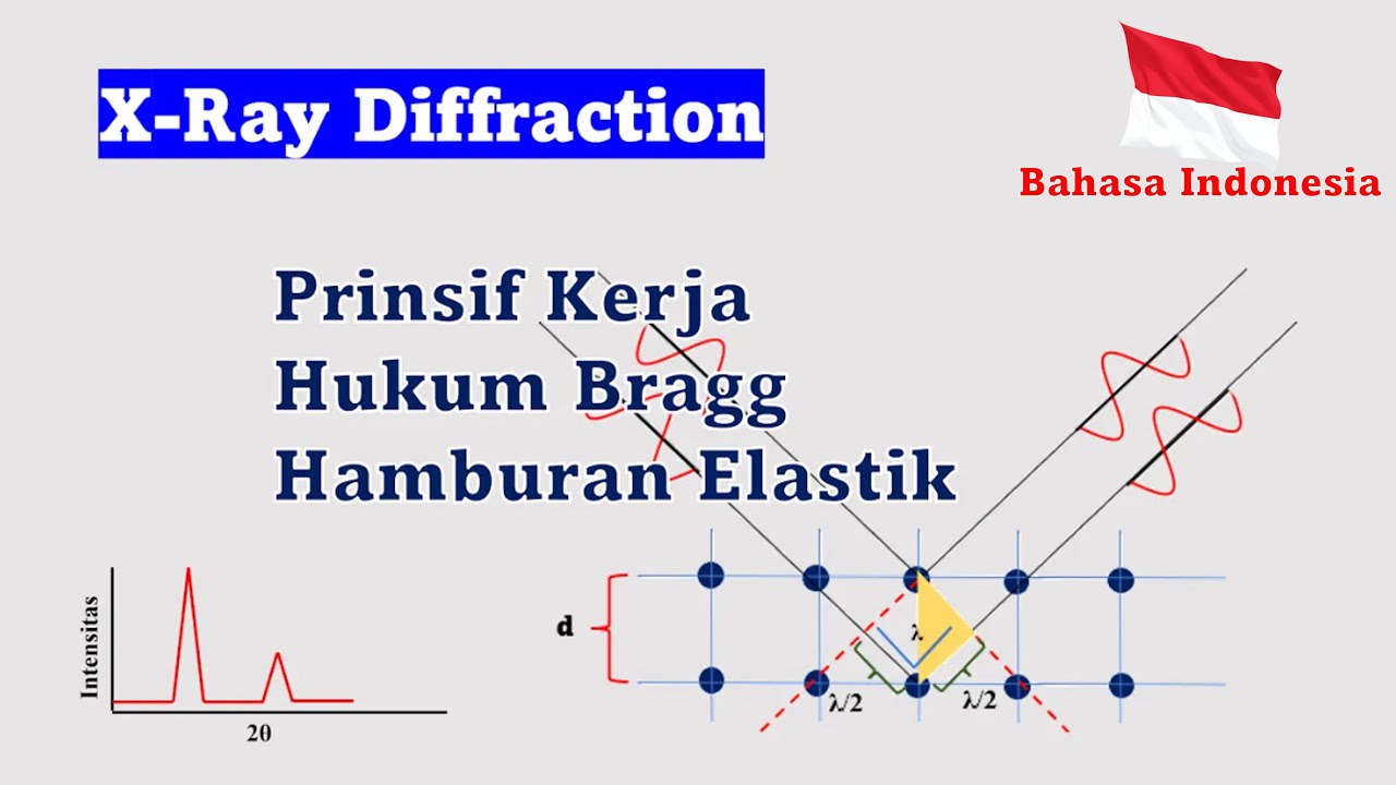
Prinsip Kerja XRD (X-Ray Diffraction) | Hukum Bragg | Bahasa Indonesia
PSPA Blok IV - 03 KLromatografi Lapis Tipis
Prosedur Analisa Logam dengan Instrumen AAS GBC (Software AAS GBC)
Session 2 Culturing Bacteria Part 1 Plating on to agar plates
5.0 / 5 (0 votes)
