Introduction to Systems of Linear Equations

Summary

Indiana Sengupta from IIT Gandhinagar introduces the fundamentals of linear algebra, focusing on systems of linear equations. The module explores homogeneous and non-homogeneous systems, defining solutions, and illustrating concepts with concrete examples. Key insights include the structure of coefficient and augmented matrices, the relationship between non-homogeneous solutions and corresponding homogeneous solutions, and the role of fields in determining solution sets. The video also explains elementary row operations and elementary matrices, showing their use in matrix manipulation and solvability analysis. These foundations set the stage for Gaussian elimination, providing a clear pathway for systematically solving linear systems.

Takeaways

• 📚 A field F can be infinite (ℚ, ℝ, ℂ) or finite (ℤp, p prime), and system coefficients belong to this field.
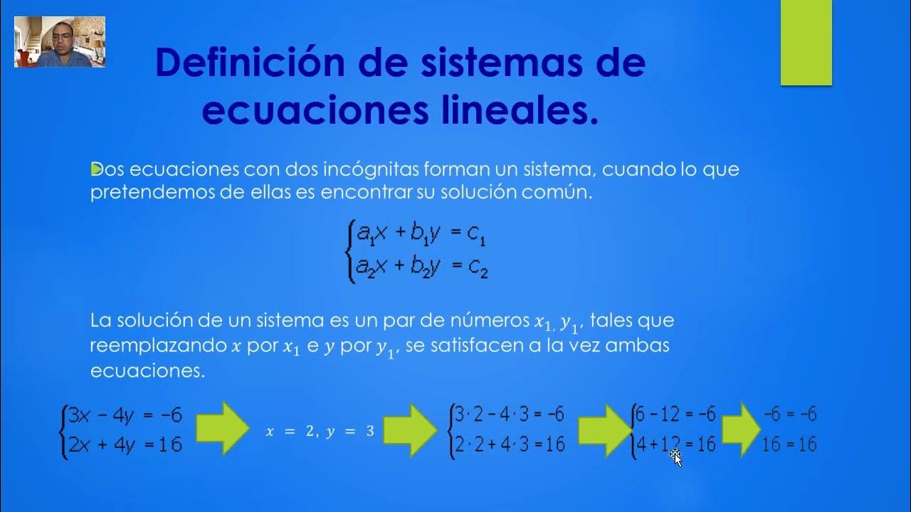
• 🧮 A system of linear equations with m equations and n unknowns can be represented in matrix form as AX = B, with an augmented matrix [A|B].
• ✅ A solution of a system is an n-tuple (α1, …, αn) satisfying all equations simultaneously.
• 🔹 Homogeneous systems have the form AX = 0 and always include the trivial solution (all zeros).
• 🔹 Non-homogeneous systems have AX = B with B ≠ 0, and solutions can be expressed as the sum of a particular solution and the general solution of the corresponding homogeneous system.
• ♾️ Homogeneous systems over an infinite field with at least one non-trivial solution have infinitely many solutions.
• ⚡ Elementary row operations (EROs) include row swaps, row scaling, and row addition, which are essential for manipulating matrices.
• 🔄 Applying an ERO to a matrix is equivalent to left-multiplying it by a corresponding elementary matrix.
• 🔑 Elementary matrices are invertible, and their inverses are also elementary matrices of the same type.
• 📝 Solving linear systems involves using elementary matrices and row operations, laying the foundation for Gaussian elimination.

Q & A

What is the first chapter of the course focused on?

The first chapter of the course focuses on systems of linear equations, which is divided into three main sections: homogeneous and non-homogeneous systems of linear equations, elementary row operations, and elementary matrices.

What is the meaning of the field 'F' in the context of linear equations?

In the context of linear equations, the field 'F' represents a set from which the coefficients of the system are drawn. It could be the rationals (ℚ), reals (ℝ), complex numbers (ℂ), or finite fields like ℤ_p (where p is a prime number).

How is a system of linear equations written in matrix notation?

A system of linear equations is written in matrix notation as 'A x = b', where 'A' is the matrix of coefficients, 'x' is the column matrix of unknowns, and 'b' is the column matrix of constants on the right-hand side of the equations.

What is an augmented matrix?

An augmented matrix is the matrix that combines the coefficient matrix 'A' and the column matrix 'b' of a system of linear equations. It is written as [A | b], where 'A' is the coefficient matrix and 'b' is the column of constants.

What is the solution to a system of linear equations in terms of 'F^n'?

The solution to a system of linear equations in 'F^n' is an n-tuple (α1, α2, ..., αn) where each αi is an element from the field 'F', such that substituting these values into the system satisfies all the equations simultaneously.

What does a typical solution of a system of linear equations look like?

A typical solution for a system of linear equations may be an n-tuple where all the unknowns take on specific values. In the case of infinitely many solutions, the solution can be expressed in terms of free variables, such as 'α, α, α' for a system where all variables are equal.

What is a homogeneous system of linear equations?

A homogeneous system of linear equations is a system where the right-hand side of the equations is the zero vector. It is represented as 'A x = 0', where '0' is a zero column vector.

What is the difference between homogeneous and non-homogeneous systems?

A homogeneous system has the right-hand side equal to zero ('A x = 0'), while a non-homogeneous system has non-zero constants on the right-hand side ('A x = b' where b ≠ 0). Homogeneous systems always have at least the trivial solution, whereas non-homogeneous systems may or may not have solutions.

What are elementary row operations, and why are they important?

Elementary row operations are transformations applied to the rows of a matrix that help solve systems of linear equations. There are three types: row swapping, scaling rows by a non-zero scalar, and adding multiples of one row to another. These operations are crucial for simplifying matrices and solving systems, especially using Gaussian elimination.

How does Gaussian elimination work with elementary matrices?

In Gaussian elimination, elementary row operations are applied to a matrix to simplify it to row echelon form. These operations can be represented by multiplying the matrix by elementary matrices. An elementary matrix is created by applying an elementary row operation to the identity matrix, and using these matrices helps in solving the system of linear equations.