materi matematika peminatan K13
Summary
TLDRThe video discusses the concept of binomial theory in probability, focusing on discrete and continuous random variables. It explains the differences between them, using examples such as the number of prime numbers below 9,000 and defective eggs in a purchase. The content covers how to calculate probability distributions, including cumulative distributions, using sample space and the binomial distribution formula. Additionally, it introduces methods for determining probability distributions using tables, functions, and graphs. The video emphasizes important principles, such as the total probability being less than or equal to one and cumulative probabilities being the sum of prior values.
Takeaways
- 😀 The lesson discusses the concept of binomial theory in probability distribution, focusing on random variables.
- 😀 The script explains the two types of random variables: discrete and continuous.
- 😀 Discrete random variables involve countable possibilities (e.g., the number of prime numbers less than 9,000).
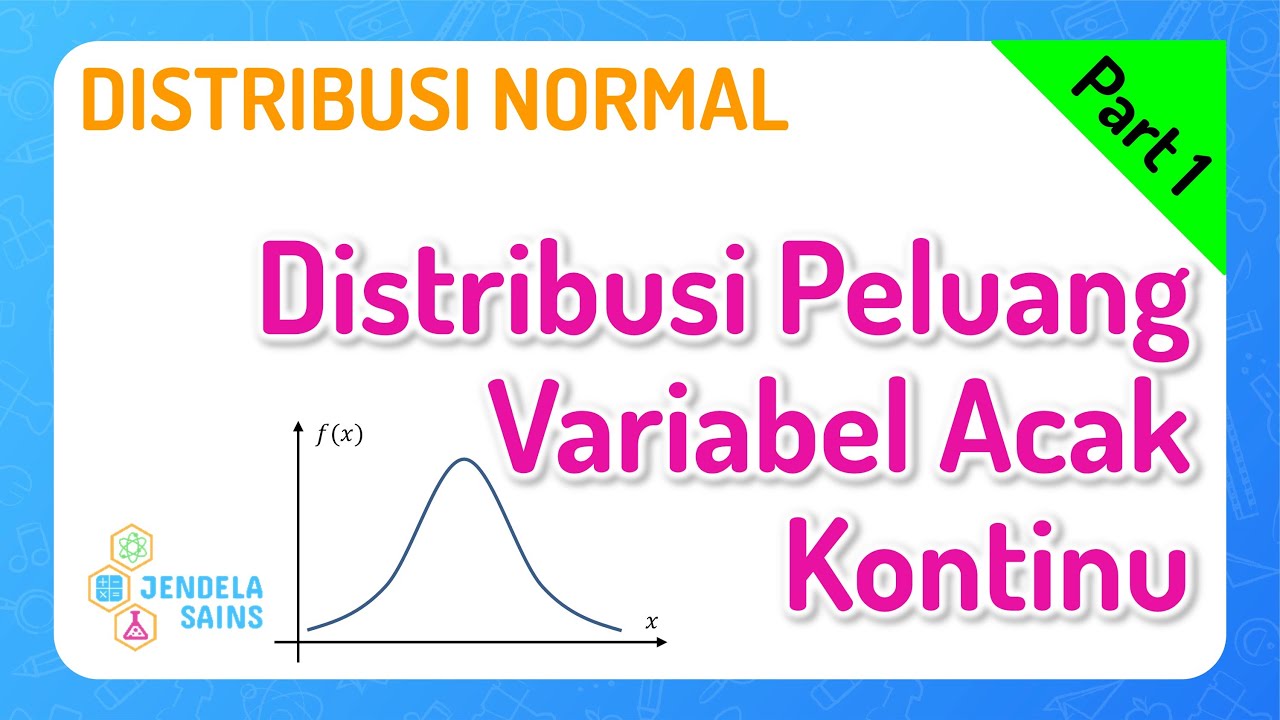
- 😀 Continuous random variables involve uncountable possibilities, such as the number of decimals between 0 and 1.
- 😀 The script illustrates examples of discrete random variables, such as counting spoiled eggs in a batch of 3 tons of eggs.
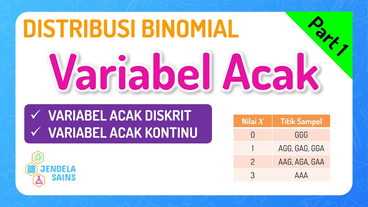
- 😀 The example of Bank Jago and its family is used to demonstrate calculating the probability distribution of random variables (e.g., the number of daughters).
- 😀 The lesson shows how to determine the probability of specific outcomes using a sample space and its possible events (e.g., no daughters, 1 daughter, etc.).
- 😀 The probability distribution for a random variable can be represented through a table, function, or graph.
- 😀 The script emphasizes that probabilities must always be between 0 and 1, and the total sum of all probabilities in a distribution equals 1.
- 😀 Cumulative distribution function (CDF) is introduced, which involves summing the probabilities of random variable outcomes up to a certain point.
Q & A
What is the main focus of today's lesson?
-The main focus of today's lesson is the probability distribution of random variables, specifically discussing discrete random variables and their cumulative distribution.
What are the two types of random variables discussed in the lesson?
-The two types of random variables discussed are discrete random variables and continuous random variables.
Can you explain what a discrete random variable is with an example?
-A discrete random variable is one that can take specific, countable values. For example, the number of prime numbers less than 9,000 is a discrete random variable because the number of primes is finite and can be counted.
What is the difference between discrete and continuous random variables?
-Discrete random variables have countable outcomes, while continuous random variables have uncountable outcomes. For instance, the number of rotten eggs in a batch is discrete, but the number of decimal values between 0 and 1 is continuous.
What is the significance of the 'Bank Jago' example in the lesson?
-The 'Bank Jago' example is used to illustrate the concept of a discrete random variable, where the random variable is the number of female children in a family, and the probabilities are calculated based on different gender combinations of the children.
How do you calculate the probability distribution for the number of female children in the 'Bank Jago' example?
-The probability distribution is calculated by determining all possible gender combinations (e.g., 0, 1, 2, or 3 female children) and finding the corresponding probabilities. For example, the probability of having 0 female children is 1/8, and the probability of having 3 female children is also 1/8.
What are the methods used to represent a probability distribution?
-A probability distribution can be represented in three ways: a table, a function, and a graph.
What does the cumulative distribution function (CDF) represent?
-The cumulative distribution function (CDF) represents the cumulative probability up to a certain point. It is the sum of all probabilities for values less than or equal to a given random variable.
How is the cumulative distribution function (CDF) calculated for the 'Bank Jago' example?
-The CDF is calculated by summing the probabilities for each value of the random variable. For example, the CDF for 0 female children is 1/8, for 1 female child is 1/8 + 3/8 = 4/8, and so on.
What is the mathematical requirement for the total probability in a probability distribution?
-The total sum of probabilities in a probability distribution must equal 1. This is because the probability of all possible outcomes must add up to certainty.
Outlines

此内容仅限付费用户访问。 请升级后访问。
立即升级Mindmap

此内容仅限付费用户访问。 请升级后访问。
立即升级Keywords

此内容仅限付费用户访问。 请升级后访问。
立即升级Highlights

此内容仅限付费用户访问。 请升级后访问。
立即升级Transcripts

此内容仅限付费用户访问。 请升级后访问。
立即升级浏览更多相关视频
Distribusi Binomial • Part 1: Variabel Acak
Distribusi Normal • Part 1: Distribusi Peluang Variabel Acak Kontinu
Introduction to Random Variables Probability Distribution
Pertemuan 1 - Distribusi Probabilitas (Part 2)

Random Variables and Probability Mass/Density Functions
Random Variable, Probability Density Function, Cumulative Distribution Function
5.0 / 5 (0 votes)
