Case Study on Regression Part I
Summary
TLDRThe video script discusses a case study on pre-owned car pricing, focusing on data analysis using Python. It covers data cleaning, handling missing values, and feature selection to develop an algorithm for price prediction. The script includes steps like importing necessary packages, data visualization, and setting parameters for features like registration year, price, and power PS. The goal is to refine the dataset for accurate car price estimations.
Takeaways
- 🚗 The case study focuses on pre-owned car pricing, aiming to develop an algorithm to predict car prices based on various features.
- 📈 Star Motors, an e-commerce company, acts as an intermediary for selling and buying used cars and has collected data from 2015 to 2016 for analysis.
- 📑 The dataset includes detailed information such as car specifications, conditions, seller details, registration information, web advertisement details, manufacturing and model information, and pricing.
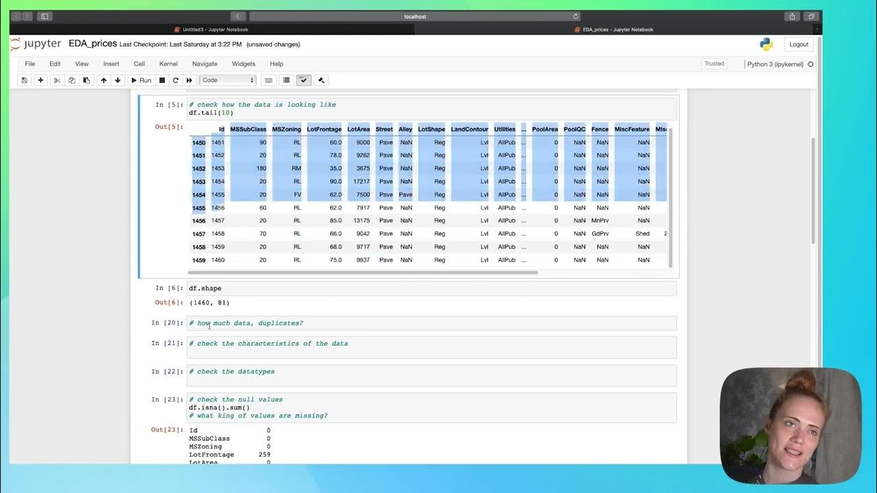
- 🛠️ The analysis involves using Python and several packages like Pandas for data manipulation and cleaning, NumPy for numerical operations, and visualization with packages like Matplotlib and Seaborn.
- 📊 Descriptive statistics and visualizations are used to understand data distribution, missing values, and the relationship between different variables like price, registration year, and engine power.
- ❓ The script discusses handling missing values and outliers, which are crucial steps in data cleaning to ensure the accuracy of the predictive model.
- 📉 The distribution of car prices shows a right-skew, indicating a long tail with higher prices, and a large variance in the data which suggests the presence of outliers.
- 🔍 Filtering and feature selection are discussed to refine the dataset for the analysis, such as removing outliers and selecting relevant features that impact car pricing.
- 📋 Data transformation techniques like scaling and normalization are considered to prepare the data for modeling, as they can influence the performance of machine learning algorithms.
- 🚀 The script emphasizes the iterative nature of data analysis, where insights from initial findings guide further data cleaning and transformation to improve the model's accuracy.
Q & A
What is the main problem discussed in the case study?
-The main problem discussed in the case study is predicting the price of used cars, specifically focusing on pre-owned cars sold by Star Motors, an e-commerce platform acting as an intermediary between sellers and buyers.
What type of data does Star Motors collect about the cars?
-Star Motors collects data on specifications, car conditions, seller details, registration details, web advertisement details, manufacturing and model information, and prices.
What specific years of data does the case study cover?
-The case study covers data from the year 2015 to 2016.
What is the goal of Star Motors in terms of algorithm development?
-Star Motors aims to develop an algorithm that helps predict the price of pre-owned cars based on various car-related features.
Which programming language is used in the case study for data analysis?
-Python is used for data analysis in the case study.
What are the initial steps taken to prepare the data for analysis?
-The initial steps include importing necessary packages, performing some numerical operations, normalizing the data, and visualizing it to understand its distribution.
What does the speaker do with the 'Cars Underscore Score' CSV data?
-The speaker sets the working directory, reads the 'Cars Underscore Score' CSV data into a DataFrame, and then explores the data to understand its structure and contents.
How does the speaker handle missing values in the data?
-The speaker creates a copy of the data to work with and then uses various functions to identify and handle missing values in different columns of the dataset.
What is the approach taken to clean the data?
-The data cleaning approach includes identifying and removing irrelevant features, handling missing values, and focusing on a specific range of data that is relevant to the analysis.
What visualization techniques are used to understand the data distribution?
-The speaker uses histograms, box plots, and scatter plots to visualize the distribution of data and understand the relationships between different variables.
How does the speaker decide on the range of data to be used for the model?
-The speaker decides on the range of data to be used for the model by considering the distribution of the data, removing outliers, and focusing on a range that is representative of the majority of the data points.
Outlines

此内容仅限付费用户访问。 请升级后访问。
立即升级Mindmap

此内容仅限付费用户访问。 请升级后访问。
立即升级Keywords

此内容仅限付费用户访问。 请升级后访问。
立即升级Highlights

此内容仅限付费用户访问。 请升级后访问。
立即升级Transcripts

此内容仅限付费用户访问。 请升级后访问。
立即升级浏览更多相关视频
EDA - part 1

Don't Buy a Car Until You Watch THIS Video | How to Negotiate a Used Car 2023
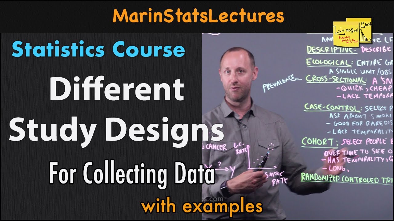
Study Designs (Cross-sectional, Case-control, Cohort) | Statistics Tutorial | MarinStatsLectures

Tipe Data dan Variabel - Google Colab - Belajar Python Pemula - Eps.3
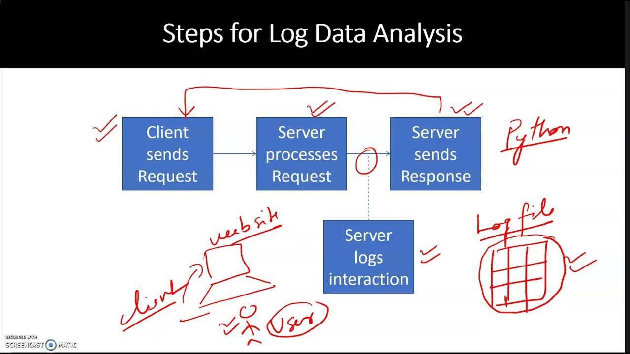
Data Analysis Processing Web Log Data

Introduction to Python for Data Science
5.0 / 5 (0 votes)
