Praktikum Sistem Daya Elektrik Percobaan I (Transmisi Pendek)
Summary
TLDRThis video script discusses an experiment on short electrical transmission lines, aiming to understand their characteristics under loaded and unloaded conditions. It explains the parameters affecting transmission line performance: resistance (R), inductance (L), capacitance (C), and conductance (G). The script covers the calculation of these parameters and their distribution along the line. It also classifies transmission lines into short, medium, and long based on their length and capacitance to ground. The video further delves into the analysis of current and voltage relationships, matrix representation, and phasor diagrams for different load conditions. Practical aspects, including the setup and data collection for modeling short transmission lines, are also addressed.
Takeaways
- 📚 The video discusses an experiment on electrical transmission systems, focusing on short transmission lines.
- 🔍 The experiment's objective is to understand the characteristics of the transmission line under loaded and unloaded conditions.
- ⚙️ Four parameters influence the performance of a transmission line: resistance (R), inductance (L), capacitance (C), and conductance (G).
- 🛠️ Resistance is due to the material's nature of the conductor, while inductance arises from the coiling of the transmission wire.
- 🌐 Capacitance is a result of the dielectric material (like air) between two electrodes, and it can be calculated using the formula C = ε₀ * A / d.
- 🔗 Conductance is the reciprocal of resistance and can be calculated using the formula G = 1/R, where R is the resistance.
- 📊 Transmission lines are classified into short, medium, and long lines based on their capacitance to ground and their length.
- 🔌 Short transmission lines are generally less than 80 km, medium lines range from 80 km to 250 km, and long lines are over 250 km.
- 📈 The video explains the equivalent circuit of a short transmission line and how to analyze it using phasor diagrams for different load conditions.
- 🔬 The experiment involves measuring voltage and current under no load, pure resistive load, and resistive-inductive (RL) load conditions.
- 🔧 Practical aspects of the experiment include using an AC three-phase voltage source, a transmission line simulator, and other equipment to model the transmission line.
Q & A
What is the main objective of the experiment discussed in the script?
-The main objective of the experiment is to understand the characteristics of a short transmission line under both loaded and unloaded conditions.
What are the four parameters that affect the performance of a transmission line as part of an electrical power system?
-The four parameters that affect the performance of a transmission line are resistance (R), inductance (L), capacitance (C), and conductance (G).
How is resistance in a transmission line related to the material of the conductor?
-Resistance in a transmission line arises due to the resistive nature of the conductor material, and it is calculated as the resistive material constant multiplied by the length of the conductor divided by its cross-sectional area.
What is the physical meaning of inductance in a transmission line?
-Inductance in a transmission line represents the property of the circuit that relates the voltage due to changes in magnetic flux to changes in current, and it is due to the coiling of the transmission wire.
How is capacitance in a transmission line affected by the dielectric material between the conductors?
-Capacitance in a transmission line is due to the presence of a dielectric material, such as air, between two electrodes, which in this case are the transmission wires and the ground. It is calculated as the permittivity of the air multiplied by the cross-sectional area of the conductor divided by the distance between the conductor and the ground.
What is conductance and how is it related to resistance?
-Conductance is the reciprocal of resistance and is calculated as the conductive material constant, where R is the resistance, which is the resistive material constant multiplied by the length of the conductor and divided by its cross-sectional area.
How are transmission lines classified based on their capacitance to ground?
-Transmission lines are classified into three types based on their capacitance to ground: short transmission lines, medium transmission lines, and long transmission lines. Short lines generally have a length of less than 80 km, medium lines range from 80 km to 250 km, and long lines are longer than 250 km.
Why can the capacitance of a short transmission line be ignored compared to the current to the load?
-The capacitance of a short transmission line can be ignored because its value is small, resulting in a very small leakage current to the ground compared to the current that goes to the load.
What is the equivalent circuit of a short transmission line as discussed in the script?
-The equivalent circuit of a short transmission line includes parameters such as sending-end voltage (Vs), receiving-end voltage (VR), DC sending current (Is), load impedance (ZL), and the line impedance (Z), which is the centralized impedance of the impedances along the line.
How are the relationships between current and voltage in a transmission line analyzed?
-The relationships between current and voltage in a transmission line are analyzed by first examining the line's equivalent circuit, considering there are no branches, so the sent current (Is) is the same as the current through the line (I_line), and the sent voltage (Vs) is equal to the voltage along the line (V_line).
What are the three conditions analyzed in the script for the transmission line's phasor diagram?
-The three conditions analyzed for the transmission line's phasor diagram are no load, loaded with R, and loaded with RL.
Outlines

此内容仅限付费用户访问。 请升级后访问。
立即升级Mindmap

此内容仅限付费用户访问。 请升级后访问。
立即升级Keywords

此内容仅限付费用户访问。 请升级后访问。
立即升级Highlights

此内容仅限付费用户访问。 请升级后访问。
立即升级Transcripts

此内容仅限付费用户访问。 请升级后访问。
立即升级浏览更多相关视频

V-I characteristics of ordinary p-n junction diode.
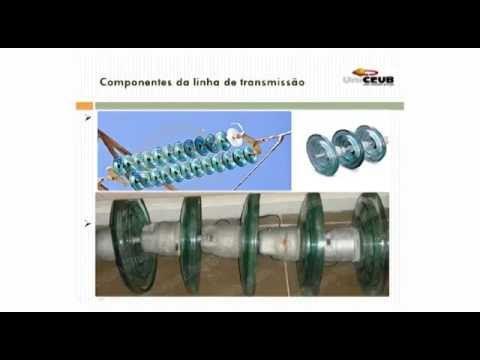
A-13 TRANSMISSÃO DE ENERGIA ELÉTRICA : AVALIAÇÃO DOS ISOLADORES

TDT01: Introduction to Transmission Lines

SGP101 Need for Protection Systems
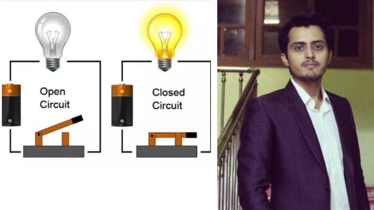
Open circuit | closed circuit | Short circuit | Easiest way to understand
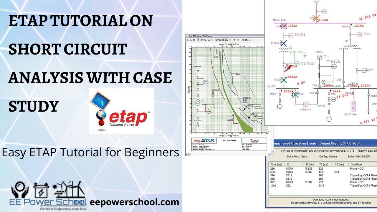
ETAP Tutorial on Short Circuit Analysis with Case Study | Easy ETAP Tutorial for Beginners
5.0 / 5 (0 votes)
