This equation will change how you see the world (the logistic map)

Summary

This video explores the surprising connections between diverse phenomena like dripping faucets, rabbit populations, thermal convection, and neuron firing, all governed by a simple logistic equation. It delves into the concept of chaos theory, illustrating how small changes can lead to unpredictable outcomes. The script discusses the logistic map's journey from stable equilibrium to chaotic behavior as growth rates increase, and how this pattern mirrors the Mandelbrot set's fractal structure. The video also highlights the Feigenbaum constant, a universal ratio observed in bifurcation processes, emphasizing the profound impact of a simple equation across various scientific fields.

Takeaways

• 📈 The logistic map is a simple equation that models population growth with environmental constraints, leading to complex behaviors like equilibrium and chaos.
• 🐰 The population of rabbits can be modeled using the logistic map, where the growth rate and initial population size affect long-term behavior.
• 🔢 The logistic map equation can lead to stable equilibrium, periodic oscillations, and chaotic behavior depending on the growth rate parameter.
• 🔁 Period doubling is a phenomenon where a system transitions from a stable state to oscillating between two, then four, and so on, values before becoming chaotic.
• 🌀 The bifurcation diagram, which shows the stable states of a system over a range of parameters, resembles a fractal and is part of the Mandelbrot set.
• 🌐 The Mandelbrot set is a famous fractal based on the iteration of a complex equation, and it includes the bifurcation diagram within its structure.
• 🔬 Scientific experiments have confirmed the logistic map's predictions in various fields, including fluid dynamics, eye response to flickering lights, and heart fibrillation.
• 💧 The dripping faucet is an example of a system that can exhibit period doubling and chaos, challenging the perception of its regularity.
• 🔢 The Feigenbaum constant (approximately 4.669) is a universal constant that describes the rate at which bifurcations occur in systems with single-hump functions.
• 🌐 Universality in chaos theory suggests that similar behaviors and constants appear across different systems and equations, indicating a fundamental aspect of nature.
• 📚 The logistic map and its implications have been influential in scientific research, prompting a call for teaching these concepts to students to foster a deeper understanding of complexity from simplicity.

Q & A

What is the logistic map equation used for modeling population growth?

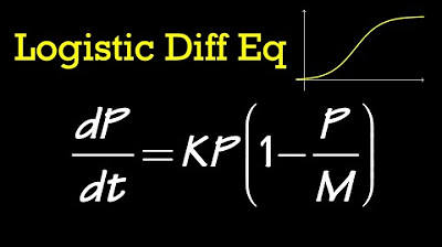
The logistic map equation is used for modeling population growth by considering both the growth rate and the carrying capacity of the environment. It is given by the formula x_{n+1} = R * x_n * (1 - x_n), where x_n is the population at time 'n', and 'R' is the growth rate.

Why does the simple exponential growth model fail to accurately represent real-world population growth?

The simple exponential growth model fails because it suggests that the population would grow indefinitely, which is unrealistic. The logistic map introduces a term to represent environmental constraints, preventing the population from exceeding the carrying capacity.

What is the significance of the value 'R' in the logistic map equation?

The value 'R' in the logistic map equation represents the growth rate of the population. It is a key parameter that influences the behavior of the population over time, including whether the population stabilizes, oscillates, or enters a chaotic state.

How does the logistic map equation demonstrate a negative feedback loop?

The logistic map demonstrates a negative feedback loop through the term (1 - x_n). As the population size x_n approaches the carrying capacity, this term approaches zero, thus reducing the growth rate and preventing the population from exceeding the environmental limits.

What is the Feigenbaum constant and what does it represent?

The Feigenbaum constant, approximately 4.669, represents the universal ratio at which bifurcations occur in systems that exhibit period doubling as they approach a chaotic state. It is a fundamental constant found in many different mathematical and physical systems.

What is a bifurcation diagram and how is it related to the logistic map?

A bifurcation diagram is a graphical representation of the stable states of a system as a function of a bifurcation parameter. In the context of the logistic map, it shows how the equilibrium population changes with the growth rate 'R', revealing patterns of period doubling and chaos.

How does the logistic map equation relate to the Mandelbrot set?

The logistic map equation is related to the Mandelbrot set because the bifurcation diagram of the logistic map is part of the Mandelbrot set when viewed in the complex plane. The behavior of the logistic map iterations mirrors the structure of the Mandelbrot set.

What is the connection between the logistic map and thermal convection in a fluid?

The logistic map's pattern of period doubling and chaos has been experimentally observed in thermal convection in a fluid, such as in the case of a fluid dynamicist's experiment with mercury in a temperature gradient, demonstrating the universality of the logistic map's behavior in different physical systems.

How has the logistic map been applied to understand heart fibrillation in medical research?

The logistic map has been used to model the progression to heart fibrillation, showing a period doubling route to chaos in the heart's beating pattern. This understanding has been applied to develop smarter ways to deliver electrical shocks to restore normal heart rhythm.

What is the significance of the Feigenbaum constant in understanding universality in chaotic systems?

The Feigenbaum constant signifies the universality of the period-doubling route to chaos across different systems and equations. Its presence indicates a fundamental process that is independent of the specific form of the equation, suggesting a deeper underlying principle in nature.

How does the logistic map equation apply to the study of dripping faucets and their behavior?

The logistic map equation can model the behavior of dripping faucets, showing how an initially regular dripping pattern can transition into period doubling and eventually chaotic behavior as the flow rate is adjusted, demonstrating the equation's applicability to seemingly simple real-world phenomena.

Outlines

00:00

🐇 The Logistic Map and Population Dynamics

The script introduces the logistic map equation as a model for population growth, using the example of a rabbit population. It explains how the equation, which includes a growth rate and an environmental constraint, can predict population behavior over time. The video demonstrates the iterative process of the logistic map, showing how populations can stabilize at an equilibrium value or oscillate between values, leading to chaos at higher growth rates. The script also mentions a contest sponsored by Fast Hosts, offering a trip to South by Southwest for answering a question about the first website.

05:01

🔄 Period Doubling and the Path to Chaos

This paragraph delves into the phenomenon of period doubling, where a system transitions from a stable state to oscillating between two, four, eight, and so on, values before eventually reaching a chaotic state. The logistic map's behavior is illustrated with graphs showing how the equilibrium population changes with the growth rate, leading to bifurcations and chaos. The script also touches on the historical significance of the logistic map in generating pseudo-random numbers and its fractal nature, which resembles the Mandelbrot set.

10:01

🌀 Universality of Chaos and the Feigenbaum Constant

The script discusses the universality of chaotic behavior across different systems, all of which can be described by the logistic map or similar single-hump functions. It introduces the Feigenbaum constant, a fundamental ratio that approaches 4.669, which describes the rate at which bifurcations occur in these systems. The constant's universality is highlighted, as it applies to any such function, regardless of its specific form, suggesting a deeper, underlying principle in nature.

15:03

🌐 Applications of Chaos Theory in Various Fields

The final paragraph explores the wide-ranging applications of the logistic map and chaos theory in diverse scientific fields. It mentions experimental confirmations of the theory in fluid dynamics, eye response to flickering lights, heart fibrillation studies, and even dripping faucets. The script emphasizes the predictive power of chaos theory in understanding complex behaviors in seemingly simple systems and concludes with a call to incorporate such concepts into education to foster a deeper understanding of complexity in nature.

Keywords

💡Logistic Map

The logistic map is a simple mathematical equation used to model population growth. It incorporates a growth rate (R) and an environmental constraint (1-X), where X is the population as a percentage of the maximum. This map demonstrates how populations can stabilize, oscillate, or become chaotic based on the growth rate.

💡Bifurcation Diagram

A bifurcation diagram is a visual representation showing how the equilibrium population varies with the growth rate (R). It illustrates different behaviors of populations, including stable, oscillating, and chaotic states, as R changes. This diagram helps to understand the transition from order to chaos in dynamic systems.

💡Period Doubling

Period doubling refers to the phenomenon where a system's behavior changes from repeating every cycle to repeating every two cycles, and so on. This occurs in the logistic map when the growth rate (R) increases beyond certain points, leading to increasingly complex behaviors before reaching chaos.

💡Chaos

Chaos in the context of the logistic map describes a state where the population does not settle into a stable pattern but appears random and unpredictable. This happens when the growth rate (R) exceeds a critical threshold, leading to complex and seemingly disordered behavior despite being determined by a simple equation.

💡Feigenbaum Constant

The Feigenbaum constant (approximately 4.669) is a universal constant that describes the ratio at which period doublings occur as a system approaches chaos. It was discovered by physicist Mitchell Feigenbaum and signifies a fundamental property of many dynamical systems, not just the logistic map.

💡Mandelbrot Set

The Mandelbrot set is a famous fractal defined by iterating a simple complex equation. Points that remain bounded are part of the set, forming intricate and self-similar patterns. The bifurcation diagram is part of the Mandelbrot set, linking chaotic behavior in real systems to complex patterns in mathematics.

💡Fractals

Fractals are complex geometric shapes that display self-similarity at various scales. The bifurcation diagram and the Mandelbrot set are examples of fractals, showing that simple iterative processes can produce infinitely intricate and detailed patterns, relevant in both mathematics and nature.

💡Periodicity

Periodicity refers to the regular, repeating cycles observed in a system's behavior. In the logistic map, periodicity changes with the growth rate (R), transitioning from stable, single values to oscillations with increasing periods, and eventually to chaos. It's a key concept in understanding dynamic systems.

💡Complex Systems

Complex systems are systems composed of many interconnected parts, which exhibit behaviors that are not simply the sum of their parts. The logistic map and its relation to chaotic behavior exemplify how simple rules can lead to complex outcomes, relevant in fields from biology to physics.

💡Pseudo-Random Numbers

Pseudo-random numbers are numbers that appear random but are generated by deterministic processes. The logistic map can produce pseudo-random numbers when it operates in its chaotic regime, demonstrating how simple equations can generate sequences that seem random without actually being so.

Highlights

The connection between a dripping faucet, the Mandelbrot set, a population of rabbits, thermal convection in a fluid, and the firing of neurons in the brain is explained through a simple equation.

The logistic map equation is introduced to model population growth, represented as \( x_{n+1} = Rx_n(1 - x_n) \), where \( x \) is the population and \( R \) is the growth rate.

The logistic map equation can lead to exponential growth, but adding a term \( 1 - X \) introduces environmental constraints, making the population a percentage of the theoretical maximum.

An example is given with \( R = 2.6 \) and an initial population of 40% of the maximum, showing how the population stabilizes over time.

The long-term behavior of the population is more interesting than the initial conditions, as it reveals an equilibrium value that the population reaches.

Graphing the population next year versus the current year shows an inverted parabola, illustrating the negative feedback loop in the logistic map.

As the growth rate \( R \) increases, the equilibrium population also increases, but there is a critical point where the behavior changes.

Once \( R \) passes 3, the graph splits into two, indicating that the population oscillates between two values, a phenomenon observed in nature as well.

As \( R \) continues to increase, period doubling bifurcations occur, leading to cycles of different lengths before eventually reaching chaos at \( R = 3.57 \).

The logistic map equation was one of the first methods used to generate random numbers on computers, providing pseudo-random numbers.

Surprisingly, order can return amidst chaos in the logistic map, with windows of stable periodic behavior appearing at certain values of \( R \).

The bifurcation diagram of the logistic map resembles a fractal, with large-scale features repeating on smaller scales.

The bifurcation diagram is part of the Mandelbrot set, showing a connection between the logistic map and this famous fractal.

The Mandelbrot set is based on an iterated equation in the complex plane, determining whether a number remains finite or goes to infinity.

The Feigenbaum constant, approximately 4.669, is a fundamental constant of nature, describing the ratio of bifurcation widths in the logistic map.

The logistic map and its bifurcation diagram have been experimentally confirmed in various scientific fields, including fluid dynamics and heart fibrillation.

The dripping faucet is an example of a system that can exhibit chaotic behavior, with period doubling observed as the flow rate increases.

The logistic map equation and its implications have been influential in scientific research, with Robert May's paper sparking a revolution in understanding complex behaviors from simple equations.

Transcripts

what's the connection between a dripping

faucet the Mandelbrot set a population

of rabbits thermal convection in a fluid

and the firing of neurons in your brain

it's this one simple equation this video

is sponsored by fast hosts who are

offering UK viewers the chance to win a

trip to South by Southwest if they can

answer my question at the end of this

video so stay tuned for that let's say

you want to model a population of

rabbits if you have X rabbits this year

how many rabbits will you have next year

well the simplest model I can imagine is

where we just multiplied by some number

the growth rate R which could be say 2

and this would mean the population would

double every year and the problem with

that is it means the number of rabbits

would grow exponentially forever

so I can add the term 1 minus X to

represent the constraints of the

environment and here I'm imagining the

population X is a percentage of the

theoretical maximum so it goes from 0 to

1 and as it approaches that maximum then

this term goes to 0 and that constrains

the population so this is the logistic

map xn plus 1 is the population next

year and xn is the population this year

and if you graph the population next

year versus the population this year you

see it is just an inverted parabola it's

the simplest equation you can make that

has a negative feedback loop the bigger

the population gets over here the

smaller it'll be the following year so

let's try an example let's say we're

dealing with a particularly active group

of rabbits so R equals two point six and

then let's pick a starting population of

40% of the maximum so point four and

then times 1 minus 0.4 and we get 0.62

four okay so the population increased in

the first year but what we're really

interested in is the long term behavior

of this population so we can put this

population back into the equation and to

speed things up you can actually type

two point six times answer times one -

answer get point six one so the

population dropped a little hit it again

point six one nine point six one three

point six one seven point six one five

point six one six point six one five and

if I keep hitting Enter here you see

that the population doesn't really

change it has stabilized which matches

what we see in the wild populations

often remain the same as long as births

and deaths are balanced now I want to

make a graph of this iteration you can

see here that it's reached an

equilibrium value of point six one five

now what would happen if I change the

initial population I'm just going to

move this slider here and what you see

is the first few years change but the

equilibrium population remains the same

so we can basically ignore the initial

population so what I'm really interested

in is how does this equilibrium

population vary depending on are the

growth rate so as you can see if I lower

the growth rate the equilibrium

population decreases that makes sense

and in fact if R goes below one well

then the population drops and eventually

goes extinct so what I want to do is

make another graph where on the x axis I

have R the growth rate and on the y axis

I'm plotting the equilibrium population

the population you get after many many

many generations okay for low values of

R we see the populations always go

extinct so the equilibrium value is zero

but once our hits 1 the population

stabilizes on to a constant value and

the higher R is the higher the

equilibrium population

so far so good but now comes the weird

part

once our passes three the graph splits

in two why what's happening well no

matter how many times you iterate the

equation it never settles on to a single

constant value instead it oscillates

back and forth between two values one

year the population is higher the next

year lower and then the cycle repeats

the cyclic nature of populations is

observed in nature too one year there

might be more rabbits and then fewer the

next year and more again the year after

as our continues to increase the fork

spreads apart and then each one splits

again

now instead of oscillating back and

forth between two values populations go

through a four year cycle before

repeating since the length of the cycle

or period has doubled these are known as

period doubling bifurcation z' and as R

increases further there are more period

doubling bifurcation z' they come faster

and faster leading to cycles of 8 16 32

64 and then at R equals three point five

seven chaos the population never settles

down at all it bounces around as if at

random in fact this equation provided

one of the first methods of generating

random numbers on computers it was a way

to get something unpredictable from a

deterministic machine there is no

pattern here no repeating of course if

you did know the exact initial

conditions you could calculate the

values exactly so they are considered

only pseudo-random numbers now you might

expect the equation to be chaotic from

here on out but as R increases order

returns there are these windows of

stable periodic behavior amid the chaos

for example at R equals 3 point 8 3

there is a stable cycle with a period of

3 years and as R continues to increase

it splits into 6 12 24 and so on before

returning to chaos in fact this one

equation contains periods of every

length 3750 1052 whatever you like if

you just have the right value

are looking at this bifurcation diagram

you may notice that it looks like a

fractal the large-scale features look to

be repeated on smaller and smaller

scales and sure enough if you zoom in

you see that it is in fact a fractal

arguably the most famous fractal is the

Mandelbrot set the plot twist here is

that the bifurcation diagram is actually

part of the Mandelbrot set how does that

work well quick recap on the Mandelbrot

set it is based on this iterated

equation so the way it works is you pick

a number C any number in the complex

plane and then start with Z equals 0 and

then iterate this equation over and over

again if it blows up to infinity well

then the number C is not part of the set

but if this number remains finite after

unlimited iterations well then it is

part of the Mandelbrot set so let's try

for example C equals 1 so we've got 0

squared plus 1 equals 1 then 1 squared

plus 1 equals 2 2 squared plus 1 equals

5 5 squared plus 1 equals 26 so pretty

quickly you can see that with C equals 1

this equation is going to blow up so the

number 1 is not part of the Mandelbrot

set what if we try C equals negative 1

well then we've got 0 squared minus 1

equals negative 1 negative 1 squared

minus 1 equals 0 and so we're back to 0

squared minus 1 equals negative 1 so we

see that this function is going to keep

oscillating back and forth between

negative 1 and 0 and so it'll remain

finite and so C equals negative 1 is

part of the Mandelbrot set now normally

when you see pictures of the Mandelbrot

set it just shows you the boundary

between the numbers that cause this

iterated equation to remain finite and

those that cause it to blow up but it

doesn't really show you how these

numbers stay finite so what we've done

here is actually iterated that equation

thousands of times and then plotted on

the z

axis the value that that iteration

actually takes so if we look from the

side what you'll actually see is the

bifurcation diagram it is part of this

Mandelbrot set so what's really going on

here well what this is showing us is

that all of the numbers in the main

cardioid they end up stabilizing on to a

single constant value but the numbers in

this main bulb will they end up

oscillating back and forth between two

values and in this bulb they end up

oscillating between four values they've

got a period of four and then eight and

then 16 32 and so on and then you hit

the chaotic part the chaotic part of the

bifurcation diagram happens out here on

what's called the needle of the

Mandelbrot set where the Mandelbrot set

gets really thin and you can see this

medallion here that looks like a smaller

version of the entire Mandelbrot set

well that corresponds to the window of

stability in the bifurcation plot with a

period of three now the bifurcation

diagram only exists on the real line

because we only put real numbers into

our equation but all of these bulbs off

of the main cardioid well they also have

periodic cycles of for example 3 or 4 or

5 and so you see these repeated ghostly

images if we look in the z axis

effectively they're oscillating between

these values as well

personally I find this extraordinarily

beautiful but if you're more practically

minded you may be asking but does this

equation actually model populations of

animals and the answer is yes

particularly in the controlled

environment scientists have set up in

labs what I find even more amazing is

how this one simple equation applies to

a huge range of totally unrelated areas

of science the first major experimental

confirmation came from a fluid

dynamicists named Lib Taber he created a

small rectangular box with mercury

inside and he used a small temperature

gradient to induce convection just two

counter-rotating cylinders of fluid

inside his box that's all the box was

large enough for and of course he

couldn't look in and see what the fluid

was doing so he measured the temperature

using a probe in the top and what he saw

was a regular spike a periodic spike in

the temperature that's like when the

logistic equation converges on a single

value but as he increased the

temperature gradient a wobble developed

on those rolling cylinders at half the

original frequency the spikes in

temperature were no longer the same

height instead they went back and forth

between two different heights he had

achieved period two and as he continued

to increase the temperature

he saw period doubling again now he had

four different temperatures before the

cycle repeated and then eight this was a

pretty spectacular confirmation of the

theory in a beautifully crafted

experiment but this was only the

beginning

scientists have studied the response of

our eyes and salamander eyes to

flickering lights and what they find is

a period doubling that once the light

reaches a certain rate of flickering our

eyes only respond to every other flicker

it's amazing in these papers to see the

bifurcation diagram emerge albeit a bit

fuzzy because it comes from real-world

data

in another study scientists gave rabbits

a drug that sent their hearts into

fibrillation

I guess they felt there were too many

rabbits out there I mean if you don't

know what fibrillation is it's where

your heart beats in an incredibly

irregular way and doesn't really pump

any blood so if you don't fix it you die

but what they found was on the path to

fibrillation

they found the period doubling route to

chaos the rabbits started out with a

periodic beat and then it went into a

two cycle two beats close together and

then a four cycle four different beats

before it repeated again and eventually

a periodic behavior now it was really

cool about this study was they monitored

the heart in real time and used chaos

theory to determine when to apply

electrical shocks to the heart to return

it to periodicity and they were able to

do that successfully

so they used chaos to control a heart

and figure out a smarter way to deliver

electric shocks to set it beating

normally again that's pretty amazing and

then there is the issue of the dripping

faucet most of us of course think of

dripping faucets as very regular

periodic objects but a lot of research

has gone into finding that once the flow

rate increases a little bit you get

period doubling so now the drips come

two at a time to tip to tip and

eventually from a dripping faucet you

can get chaotic behavior just by

adjusting the flow rate and you think

like what really is a faucet well

there's constant pressure water and a

constant size aperture and yet what

you're getting is chaotic dripping so

this is a really easy chaotic system you

can experiment with at home go open a

tap just a little bit and see if you can

get a periodic dripping in your house

the bifurcation diagram pops up in so

many different places that it starts to

feel spooky and I want to tell you

something that'll make it seem even

spookier

there was this physicist Mitchell

Feigenbaum who was looking at when the

bifurcations occur he divided the width

of each bifurcation section by the next

one and he found that ratio closed in on

this number four point six six nine

which is now called the Feigenbaum

constant the bifurcations come faster

and faster but in a ratio that

approaches this fixed value and no one

knows where this constant comes from it

doesn't seem to relate to any other

known physical constant so it is itself

a fundamental constant of nature what's

even crazier is that it doesn't have to

be the particular form of the equation I

showed you earlier

any equation that has a single hump if

you iterate it the way that we have so

you could use xn plus 1 equals sine X

for example if you iterate that one

again and again and again you will also

see bifurcations not only that but the

ratio of when those bifurcations occur

will have the same scaling for point six

six nine any single hump function

iterated will give you that fundamental

constant so why is this well it's

referred to as universality because

there seems to be something fundamental

and very Universal about this process

this type of equation and that constant

value in 1976 the biologist Robert May

wrote a paper in nature about this very

equation

it's sparked a revolution and people

looking into this stuff I mean that

papers been cited thousands of times and

in the paper he makes this plea that we

should teach students about this simple

equation because it gives you a new

intuition for ways in which simple

things simple equations

can create very complex behaviors and I

still think that today we don't really

teach this way I mean we teach simple

equations and simple outcomes because

those are the easy things to do and

those are the things that make sense

we're not gonna throw chaos at students

but maybe we should maybe we should

throw at least a little bit which is why

I've been so excited about chaos and I

am so excited about this equation

because you know how did I get to be 37

years old without hearing of the

Feigenbaum constant ever since I read

James Gleeks book chaos I have wanted to

make videos on this topic and now I'm

finally getting around to it and

hopefully I'm doing this topic justice

because I find it incredibly fascinating

and I hope you do too hey this video is

supported by viewers like you on patreon

and by fast hosts fast toasts is a

uk-based web hosting company whose goal

is to support UK businesses and

entrepreneurs at all levels providing

effective and affordable hosting

packages to suit any need for example

they provide easy registration for a

huge selection of domains with powerful

management features included plus they

offer hosting with unlimited bandwidth

and smart SSD storage they ensure

reliability and security using clustered

architecture and data centers in the UK

now if you are also in the UK you can

win two tickets to South by Southwest

including flights and accommodation if

you can answer my text question which is

which research organisation created the

first website if you can answer that

question then enter the competition by

clicking the link in the description and

you could be going to South by Southwest

courtesy of fast hosts their data

centers are based alongside their

offices in the UK so whether you go for

a lightweight web hosting package or a

fully fledged dedicated box you can talk

to their expert support teams 24/7 so I

want to thank fast hosts for supporting

veritasium and I want to thank you for

watching