Materi Kuliah Model Simulasi: Pembangkit Random Variate Kontinu
Summary
TLDRThis video explains the process of solving problems related to continuous random variables using integration and random number generation. The speaker discusses how to determine the cumulative distribution function (CDF) of a given function, find its probability density, and solve quadratic equations using the ABC formula. Additionally, the process includes applying random numbers to generate possible outcomes and calculating averages for optimal solutions. Key concepts covered include integral calculus, quadratic equations, and random variable simulations, offering a comprehensive guide for statistical problem-solving.
Takeaways
- 😀 The video covers the concept of random variables, focusing on both discrete and continuous types.
- 😀 The importance of calculating the cumulative distribution function (CDF) for continuous random variables is emphasized.
- 😀 The process of solving for CDF is explained using integral methods, specifically when the data is distributed continuously.
- 😀 An example function FX = 3x + 1 is used to demonstrate the calculation of the probability density function (PDF) and the CDF.
- 😀 To solve for the CDF, the integral of the given function is computed, with the results forming the foundation for determining probabilities.
- 😀 The script explains how to solve a quadratic equation using the quadratic formula (ABC formula) to determine the value of x in a continuous distribution.
- 😀 A random number is then used to calculate corresponding values for the random variable X.
- 😀 A second example function, FX = a(1 - x) where x is between 0 and 1, is introduced, with the task of determining the CDF and solving for the constant 'a'.
- 😀 The CDF for this second example is derived using the same integral method, with 'a' being determined to be 2 for the equation to hold true.
- 😀 The relationship between CDF and random numbers is explored, showing how to substitute random numbers into the CDF to generate corresponding values for X.
- 😀 The script concludes with instructions on how to compute and average the random variable values to determine an optimal solution using the derived formulas.
Q & A
What is the first step in solving for a continuous random variable as described in the script?
-The first step is determining the CDF (Cumulative Distribution Function) using integration if the data is known to follow a continuous distribution.
What formula is used to calculate the CDF in the script?
-The CDF is calculated by integrating the probability density function (PDF) using the formula: ∫ f(x) dx.
How is the probability density function (PDF) derived in the script?
-The PDF is derived by taking the integral of the function FX(x), and then calculating the constant terms as necessary, such as using basic integration rules.
What method is used to solve the quadratic equation obtained in the CDF integration process?
-The quadratic equation is solved using the quadratic formula (x = (-b ± √(b² - 4ac)) / 2a), where the coefficients are substituted from the equation.
Why is the quadratic formula used in this process?
-The quadratic formula is used because the resulting equation after integrating the PDF leads to a quadratic form, which can be solved for the random variable values.
What is the significance of the random numbers (R1, R2, etc.) in the process?
-Random numbers are used to generate specific values for the continuous random variable, which are obtained by substituting these numbers into the equation derived from the CDF.
How do you connect the CDF to random numbers in the script?
-The connection is made by substituting the generated random numbers into the equation obtained from the CDF. The results help in determining specific values for the random variable.
How are the solutions for X1 and X2 determined in the second part of the script?
-The solutions for X1 and X2 are determined by solving the quadratic equation formed after substituting the random numbers into the CDF equation. The values are then averaged to find the optimal solutions.
What role does the constant 'a' play in the second example with the function 'a * (1 - x)'?
-The constant 'a' in the second example is determined by solving for it through integration, ensuring that the resulting CDF equals 1, as required for a valid probability distribution.
What happens after the values for X1 and X2 are obtained using the random numbers?
-After the values for X1 and X2 are obtained, the next step is to calculate their averages to find the optimal values for the random variables.
Outlines

This section is available to paid users only. Please upgrade to access this part.
Upgrade NowMindmap

This section is available to paid users only. Please upgrade to access this part.
Upgrade NowKeywords

This section is available to paid users only. Please upgrade to access this part.
Upgrade NowHighlights

This section is available to paid users only. Please upgrade to access this part.
Upgrade NowTranscripts

This section is available to paid users only. Please upgrade to access this part.
Upgrade NowBrowse More Related Video

Random Variables - Grade 11 (Statistics and Probability) @MathTeacherGon

Random Variable, Probability Density Function, Cumulative Distribution Function

Random Variables and Probability Distributions

VARIABEL ACAK DISKRIT: Pengertian dan Distribusi Peluang-nya!
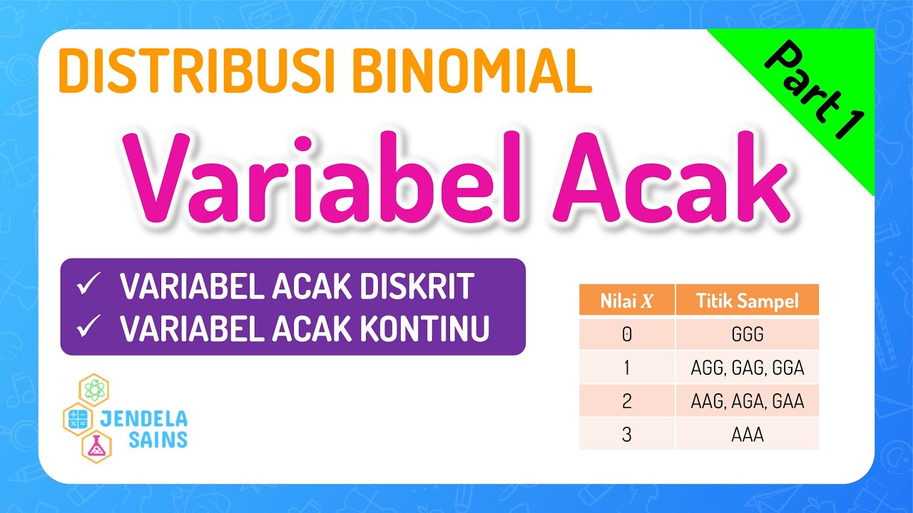
Distribusi Binomial • Part 1: Variabel Acak

Discrete and continuous random variables | Probability and Statistics | Khan Academy
5.0 / 5 (0 votes)