Queuing theory and Poisson process

Summary

This script explores queuing theory, focusing on the Poisson process to model customer arrivals in a queue. It simplifies the system by assuming independent arrivals and service completions, leading to the M/M/1 queue model. The script delves into the derivation of probability equations for queue states and their long-term behavior, highlighting the importance of the ratio of arrival to service rates. It concludes with the invariant distribution for stable queues and introduces more complex queuing models, providing a foundational understanding of real-life queue modeling.

Takeaways

• 📊 In real life, queues can be modeled by focusing on customer arrivals and service processes.
• 📅 Customer arrivals are assumed to be independent, arriving at random intervals.
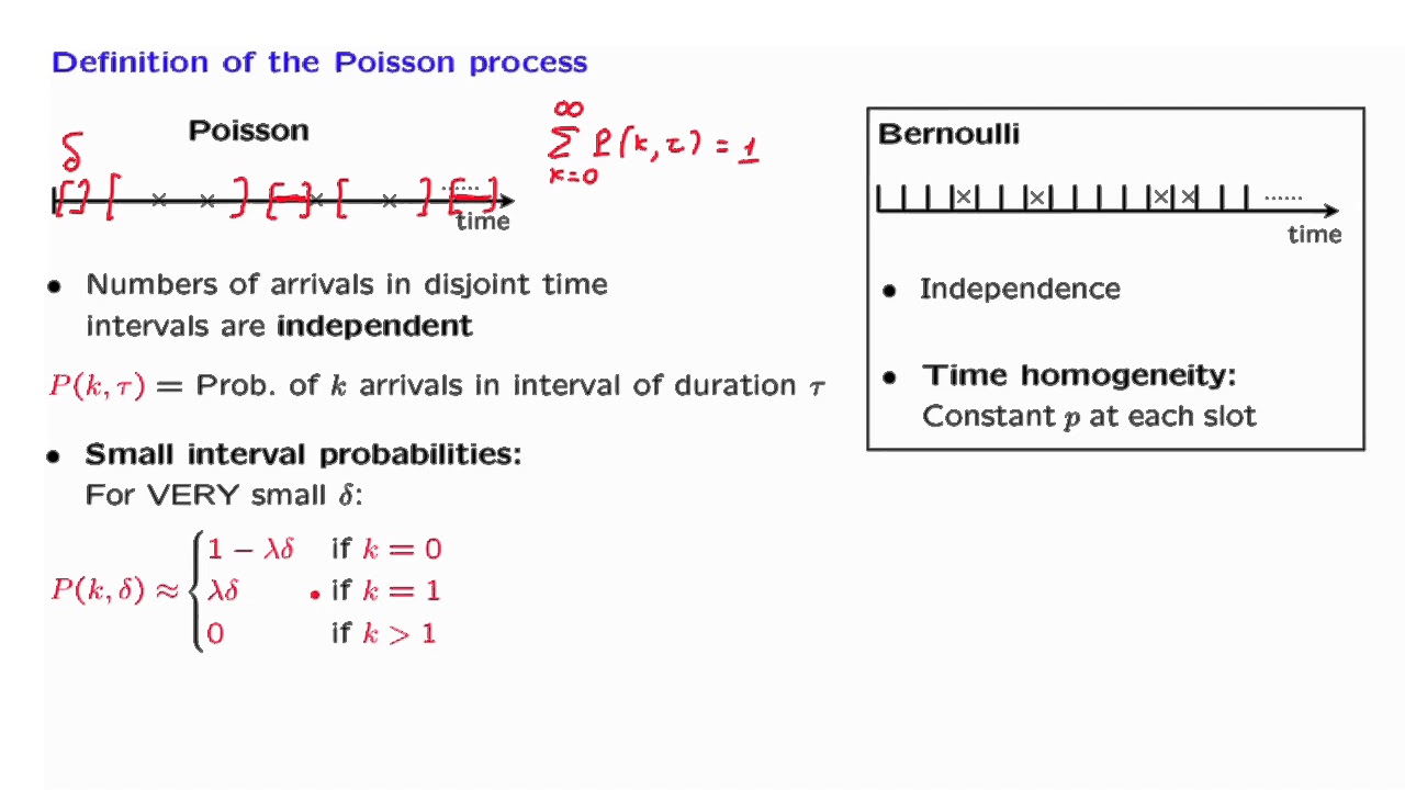
• 🔢 The Poisson process is used to model customer arrivals, with the average rate of arrivals denoted as lambda.
• 🧮 The probability of having k customers arriving in a unit time follows a Poisson distribution.
• 🔄 The service process in a queue can also be modeled with a rate of service denoted as mu, which might differ from the arrival rate.
• 📈 The state of the queue is represented by the number of customers present, evolving over time based on arrival and departure rates.
• 🧩 Differential equations describe the evolution of queue states over time, though exact solutions can be complex.
• 📉 The long-term behavior of the queue can stabilize, leading to a constant distribution of state probabilities, known as the invariant distribution.
• 💡 The simplest queuing model, M/M/1, assumes memoryless arrival and service processes, but more complex models like M/M/c or M/G/k exist.
• 🌐 Networks of queues, such as Jackson networks, involve interactions between multiple queues, adding complexity to the model.

Q & A

What is the fundamental assumption made when modeling customer arrivals in a queue?

The fundamental assumption is that the arrival times are independent from each other, meaning a customer arriving at a specific time has no knowledge about the other customers or their arrival times, essentially showing up at random.

How is the average number of customers arriving in a unit of time calculated?

The average number of customers arriving in a unit of time is calculated by multiplying the probability of a customer arriving in a subinterval (lambda / n) by the number of subintervals (n), which simplifies to lambda.

What is the Poisson distribution and how is it related to the queuing model?

The Poisson distribution is a probability distribution that expresses the probability of a given number of events occurring in a fixed interval of time. It is used in the queuing model to represent the distribution of the number of customers arriving during a unit time interval.

What is the M/M/1 queue model and what does each 'M' stand for?

The M/M/1 queue model is a type of queuing model where 'M' stands for memoryless, indicating that both the arrival process and service times are memoryless (exhibiting the property of independence between inter-arrival and service times). The '1' indicates there is only one service counter.

What is the significance of the ratio lambda/mu in the M/M/1 queue model?

The ratio lambda/mu is significant as it determines the stability of the queue. If lambda is less than mu, the queue is stable and probabilities tend to an invariant distribution. If lambda is greater than mu, the queue is unstable and tends to grow indefinitely.

What does the term 'memoryless' imply in the context of queuing theory?

In queuing theory, 'memoryless' refers to the property where the probability of an event occurring in the next time interval is independent of the time since the last event occurred. This is a characteristic of both the arrival process and service times in the M/M/1 model.

How are the long-term probabilities of the queue being in different states calculated?

The long-term probabilities are calculated by solving a set of recurrence relations derived from the differential equations governing the evolution of the probabilities. The sum of these probabilities must equal 1, which helps in finding the initial probability pi_0.

What is a Jackson network in the context of queuing theory?

A Jackson network is a queuing network model where multiple individual queues (often M/M/1 queues) interact with each other. After service, a customer can either leave the system entirely or join the back of another queue in the network.

What are the modified Bessel functions of the first kind and why are they important in the M/M/1 queue model?

The modified Bessel functions of the first kind are special functions that often appear in solutions to differential equations. In the M/M/1 queue model, they appear in the exact solution for the probabilities of the queue being in different states, making them important in the mathematical analysis of the queue.

What is the qualitative behavior of the M/M/1 queue model when lambda is greater than mu?

When lambda is greater than mu, the queue model exhibits a qualitative behavior where the queue tends to grow over time. The probabilities shift towards more customers in the queue, and the system does not stabilize at a set of invariant probabilities.

Outlines

00:00

📊 Modeling Customer Arrivals

The process of modeling customer arrivals in a queue is explained. The arrival times are independent, likened to flipping a coin in small time intervals, with a probability p of a customer arriving. By dividing time into intervals and adjusting p, we ensure an average rate of λ customers per unit time. This leads to the Poisson distribution, used to model the probability of k customers arriving in a given time.

05:03

📈 Simplifying the Queue Model

An introduction to combining the arrival and departure processes in a queuing model. Arrivals occur with rate λ and departures with rate μ, assuming they happen independently. The state of the queue is denoted by the number of customers, and the probabilities of these states evolve over time. The model is mathematically simplified but unrealistic.

10:09

🔄 Evolution of Queue Probabilities

Focuses on the evolution of state probabilities over small time intervals. For any state k, the probability pk(t) changes based on arrivals and departures. The derived equations describe how these probabilities evolve, with special consideration for state 0. As n tends to infinity, these equations transform into differential equations, giving a continuous-time model.

15:12

🧮 Solving the Differential Equations

Details the process of solving the differential equations governing the queue's state probabilities in the long term. The probabilities pk(t) tend to constants πk, forming a recurrence relation. This relation reveals that πk is a geometric sequence, converging if λ / μ < 1, indicating a stable queue. Otherwise, the queue grows indefinitely.

20:18

🔀 Long-term Queue Behaviour

Discusses the long-term behaviour of queues. If λ < μ, the queue stabilizes, leading to an invariant distribution. This distribution shows the steady-state probabilities for different queue states. However, the model's assumption of memoryless service and arrival times is unrealistic. The video concludes by introducing variations like M/M/c and M/G/k models, and the Jackson network for more complex queue interactions.

Keywords

💡Queue

A queue in the context of the video refers to a line of customers waiting for service. It is the central theme of the video, discussing how queues are modeled and analyzed. The script uses the concept of queues to explain the mathematical processes behind customer arrivals and departures.

💡Customer Arrivals

Customer arrivals represent the process of customers coming into the queue to receive service. The video script discusses modeling this process with the assumption of independent arrival times, meaning the arrival of one customer does not affect the others. This concept is foundational for the Poisson process described in the video.

💡Service

Service in the video refers to the process provided by a company to customers in the queue. It is a critical component of the queuing model, where the script explains the service rate and how it can be modeled independently from customer arrivals, with its own constant, mu.

💡Poisson Distribution

The Poisson distribution is a probability distribution that the video describes as being used to model the number of events (in this case, customer arrivals) in a fixed interval of time. It is integral to understanding the likelihood of a certain number of customers arriving during a given period.

💡Poisson Process

The Poisson process is a statistical model used to describe the occurrence of events over time, where the events occur independently and with a known average rate. In the video, it is used to model customer arrivals in a queue, assuming an average rate of lambda customers per unit time.

💡Memoryless Property

The memoryless property, as mentioned in the script, refers to the characteristic of the service times and arrival process where the probability of an event occurring is independent of the time since the last event. This property is key to the M/M/1 queue model discussed in the video.

💡M/M/1 Queue

The M/M/1 queue is a specific type of queuing model characterized by having one server (indicated by the '1'), and both the arrival and service processes are memoryless (indicated by the two 'M's). The video uses this model to illustrate the basic principles of queuing theory.

💡Departure Process

The departure process in the video refers to customers leaving the queue after receiving service. It is modeled independently from the arrival process, with its own rate, mu, and is essential for understanding the dynamics of the queue over time.

💡State of the Queue

The state of the queue is defined by the number of customers present in the system at any given time. The video script discusses how the state evolves and is crucial for understanding the queuing model, as it helps to track and predict the queue's behavior.

💡Differential Equations

Differential equations are used in the video to describe the evolution of probabilities over time in the queuing model. They are essential for understanding how the system's state changes and for deriving the long-term behavior of the queue.

💡Invariant Distribution

The invariant distribution in the video refers to the long-term limit of the probabilities of the queue being in different states. It is a key concept for understanding the steady-state behavior of the queue, where the probabilities stabilize over time.

💡Qualitative Behavior

Qualitative behavior in the context of the video refers to the general trends and characteristics of the queuing model without focusing on the exact mathematical solutions. The script discusses analyzing these behaviors, such as the invariant distribution, to understand the system's long-term tendencies.

Highlights

Modeling queues involves separating the process into customer arrivals, service provision, and customer departures.

Customer arrivals are modeled with the assumption of independent arrival times, likened to flipping a coin with a small probability p for each interval.

The average number of customers arriving in a unit of time is represented by np, where n is the number of intervals and p is the probability of arrival in each interval.

The probability p is adjusted as lambda/n to ensure an average of lambda customers arrive per unit time as the number of intervals increases.

The probability of k customers arriving in a given time is calculated using a formula involving the Poisson distribution.

The Poisson distribution is used to model the number of customers arriving in a unit time interval with an average rate of lambda.

The queuing model also incorporates the service part, with the unrealistic but mathematically simple assumption of independent service completion with a rate mu.

The state of the queue is denoted by the number of customers in the system, with state 0 indicating an empty queue.

The evolution of the queue's state probabilities over time is analyzed using differential equations derived from discrete time intervals.

The long-term behavior of the queue probabilities is studied under the assumption of system stability, leading to a constant probability for each state.

The long-term probabilities are found to form a geometric sequence, with the sum of probabilities equating to 1, given the condition lambda/mu < 1.

The condition lambda < mu ensures the queue will stabilize, as a higher arrival rate would lead to an ever-growing queue.

The model described is an M/M/1 queue, characterized by memoryless arrival and service processes and a single service counter.

More complex queuing models like M/M/c and M/G/k account for multiple service counters and non-memoryless service times, respectively.

Jackson networks represent a system of interacting queues, where customers may move between queues after service.

Qualitative behaviors such as the invariant distribution and long-term behavior are often of more interest due to the complexity of exact solutions.

The video concludes with an invitation to watch another video on the second channel for more information on the Poisson distribution.

Transcripts

In real life, we have seen a lot of queues, but how do we model them? In general, for

any queue, we can separate the process into customer arrivals, and then the company will

provide some service to the customers, and after the service, the customers will leave

the queue, and the cycle repeats. Let’s first focus on the first part: customer arrivals.

To model the customer arrivals, we make an important assumption: the arrival times are

independent from each other. And by independent arrivals, I mean that a customer arriving

at a specific time has no knowledge about the other customers nor their arrival times,

sort of showing up at random. Practically, you can think about it like this: on the timeline,

we can divide it into many subintervals. At each subinterval, it is kind of like flipping

a coin, and with some certain small probability p, there is a customer coming into the queue.

If we divided 1 unit of time into n subintervals, and at each interval, there is probability

p that a new customer shows up, then on average, we should expect there to be np number of

customers coming in 1 unit of time.

However, ultimately we would like to let n tend to infinity rather than having discrete

intervals. To make sure that we don’t end up with infinite number of customers turning

up, we adjust the probability p to change with the number of intervals, lambda / n,

so that on average, within a unit of time, we get lambda customers coming in, and that

lambda is a constant. And once we have set this up, we can analyse this as a usual probability

problem. One possible thing we might be interested in is the probability that there are k customers

coming in during this time. Each customer arrival would contribute lambda / n probability,

so there would be (lambda / n)^k probability in those intervals, but for all the other

intervals to not have customers coming in, we would have to multiply (1 - lambda / n)

(n - k) times. There could very well be other sets of intervals those k customers come in,

so we also have to multiply an extra n choose k factor to include all possible ways customers

could come in. So this is the formula for the probability of k customers coming in within

this time.

Ultimately, we would like to subdivide it into many more intervals, letting n to infinity,

so we just have to evaluate this expression when n tends to infinity. (Wait 41 seconds)

And this is the final expression that we get. This was originally the probability of getting

k customers coming in, if on average we expect the number to be lambda. So for a summary,

if we have an average rate of lambda customers coming in, the probability that there are

exactly k of them in a unit time interval is this exponential expression, which can

be put in the form of a table, making it a little more obvious that we can view it as

a distribution of the number of customers. Such a distribution is called Poisson distribution,

and the entire model of customer arrivals is called the Poisson process. So we have

modelled the customer arrivals by the Poisson process, but that’s just *part* of the queuing

model. We also have to incorporate the service part of the queue.

The model I will describe is quite unrealistic, but mathematically the simplest to work with.

I will describe other models at the end. For the arrival process, there is a lambda/n chance

of a customer coming in. We assume that at the same time, the departure process, that

is the service is finished for a customer, also happens independently with the same mechanism,

just with a potentially different constant, mu. Of course, that is when there is at least

1 customer in the system, otherwise no departure can happen. This is quite an unrealistic model,

because the duration of the service is completely determined by luck. But putting both arrival

and departure in the same framework simplifies a lot. Usually, we like to represent this

process in a more compact way.

We denote the state of the queue by how many customers there are in the system. For example,

state 0 means no customers in the queue, and the queue is clear. The customer arrives at

a rate of lambda, so it advances from state 0 to state 1 at a rate of lambda, and so on

for the other states. At the same time, by our rather unrealistic model, the customers

leave at a rate of mu, so the rate at which the number of customers go down 1 is mu. At

the start of this queuing process, we would assume that we don’t have any customers.

In other words, initially, the probability of the state being 0 is 1, but for other states,

initially the probability is 0. In general, these probabilities will evolve over time,

with the probabilities denoted as p_k(t), where that k is the state of the queue. These

values above are just the probabilities when t = 0. One possible direction for analysis

of this queue is to study the evolution of these probabilities.

For example, let’s focus on the “2” state and the neighbouring states. What happens

if we just move time forward by 1/n, one subinterval of time? There are three contributions to

this probability. First case is that at time t, it was at state 2 already, but no customers

have arrived or departed during that tiny time interval. The contribution looks something

like this: p_2 (t) denotes the probability that at the time t it was actually at state

2, and the other part is the probability that neither arrival nor departure happens within

the time between t and t + 1/n. (1 - lambda / n) is the probability of no arrival, and

(1 - mu / n) is the probability that no customers have left the queue this time. This is only

one of the possibilities - not changing the state of the queue.

The second possibility is that at time t, the queue was at state 3, but a customer left

after the service. This case contributes this term on the right. Like before, p_3(t) is

the probability at state 3 at the previous step, and mu/n is the probability that a departure

happens during this time. The final possibility is that originally it was at state 1, and

then a customer comes in during this time. The contribution would be p_1(t), the probability

that originally it was at state 1, times lambda / n, the probability that an arrival occurs.

So this expression on the right is how p_2 evolves as we increment 1 subinterval of 1/n.

But this is just focusing on the evolution of p_2. The exact same argument would apply

for any state k, so we should expect a similar equation for state k. I have literally just

replaced any instance of 2 to be k, 3 to be k+1, and 1 to be k-1. This equation works

almost all the time, except for the case when k = 0, because we can’t have -1 customer

in the queue, so this term doesn’t make sense. No worries, it just means that we need

to deal with the case k = 0 separately, and the process is very, very similar to what

we just did.

To contribute to the probability at state 0 at time t + 1/n, we can either not lucky

enough to get a customer arrival, in which case, the contribution is probability that

you were originally at state 0, times (1 - lambda / n), the probability that you haven’t got

an arrival during this time; or there was originally 1 customer in the queue, and during

this time, the service has finished and the customer left the queue. The contribution

in this case would be p_1(t) times mu / n, the probability of customer departure during

this time. So we have completed the derivation of these evolution equations from time t to

time t + 1/n, with the first equation working for almost all k, except when k = 0, and the

second equation specifically dealing with the case k = 0. As with previous discussions,

we would like to let n tend to infinity, so that we are no longer using discrete time

intervals.

Let’s focus on the first equation first and think about what happens when n tends

to infinity. The first step is to rewrite the left hand side so that it becomes like

a rate of change. For the first term, we subtract p_k(t) from it, and then multiply the term

by n, giving us p_k(t) times (- lambda - mu + lambda mu /n). And for all the other terms,

we just have to multiply by n. Finally, we just have to consider the limit of all these

as n tends to infinity. The left hand side would tend to the derivative of p_k(t). The

first term of the right hand side would tend to - (lambda + mu) p_k(t), and the remaining

two terms do not depend on n, so they tend to whatever they were before. This becomes

a differential equation in the continuous case, but this again only works when k does

not equal to 0. We just now have to deal with the case when k equals 0. This comes from

considering the limit of the second equation when n tends to infinity.

In very much the same fashion, we consider the rate of change of p_0(t). We subtract

the first term by p_0(t), and then multiply it by n, giving us - lambda p_0(t). For the

other term on the right hand side, we just multiply it by n, giving us mu p_1(t). Again,

the left hand side would tend to a derivative, in this case, p_0 prime (t), and the terms

on the right hand side do not depend on n, so they tend to whatever they were before.

This would be the differential equation coming from the case for the state 0. So altogether,

we would have these differential equations governing the evolution of these probabilities.

In theory, we could just solve them, and pretty much everything you want to know from this

queuing model falls out. However, even in this rather simple queuing model, the exact

solution looks horrible. And not only is it horrible, these I_k or I_l’s are actually

special functions called the modified Bessel functions of the first kind. To be fair, these

Bessel functions are hugely important in many different fields, including Schrodinger’s

equation, so it is not really obscure, and a lot of properties are known. Still, due

to the complexity of the exact solution, we might be better off analysing more qualitative

behaviour.

For example, what is the long-term behaviour of these probabilities? If we assume that

the system becomes stable in the long term, which means that these probabilities eventually

tend to a constant for each k, what are those pi_k’s? Well, using this assumption and

plucking it back to the differential equations, in the long run, these derivatives vanish,

and all the other p_k(t)’s can be replaced by the constants pi_k. Then we end up with

a recurrence relation between these pi_k’s. Solving this is much easier than the full

differential equation, and this is what we will do. To start with, we can rewrite the

first recurrence relation as such: (wait 15 sec) This highlights that the difference between

consecutive pi_k’s is related by a ratio of lambda / mu. What this means is that if

we have the value of pi_1 - pi_0, by multiplying lambda / mu, we get the next difference pi_2

- pi_1, and so on by multiplying lambda / mu all the way through. Making our notations

a little easier, we write the initial difference to be d, then the other of these differences

would be a power of lambda / mu, times d.

Now for example, if we know the value of pi_0, then we can obtain the value of pi_4, simply

by adding up pi_0 and these differences. The sum telescopes to pi_4. Now because we can

rewrite these differences in terms of lambda / mu, and d, in general we have that pi_k

is the sum pi_0, and the sum of these differences between consecutive terms, which are powers

of lambda / mu multiplied by d. So that’s the conclusion we draw from the recurrence

relation, but the other equation from the long-term behaviour of these probabilities

involves pi_0 and pi_1. This tells us that pi_1 is this lambda / mu times pi_0, which

means that their difference is this (lambda / mu - 1) times the initial pi_0. Because

we have denoted the difference as d, we just have to substitute this formula for d into

the previous expression for pi_k, giving pi_k in terms of pi_0 and lambda / mu only. Now

notice that this part is actually a factorisation of (lambda / mu)^k - 1, and using this observation,

we can conclude that pi_k’s are actually just a multiple of pi_0, and a power of (lambda

/ mu).

So during this quest of finding the long-term behaviour of the probabilities, solving these

recurrence relations means that the long-term probabilities should look like these at different

states. Like at state “3”, if the probabilities stabilise, then it must be pi_0 times (lambda

/ mu)^3, and so on. Finally, to fully solve this system, we actually have a bit of a hidden

assumption as these indicate probabilities. That is, the sum of these probabilities has

to be 1. Given that these probabilities form a geometric sequence, we can compute the sum

of these probabilities by the formula for a geometric series if it converges, and get

that pi_0 / (1 - lambda / mu) = 1, which in turn means that pi_0 is 1 - lambda / mu. However,

note that this geometric series only works if it converges, that is the ratio lambda

/ mu is smaller than 1. Well, to be honest, just looking at pi_0, we also know that lambda

/ mu must be smaller than 1 for this argument to make sense.

And this condition that lambda needs to be smaller than mu makes sense. If instead, lambda

is larger than mu, then on average, lambda being the average rate at which the customer

comes in, is quicker than mu, the average rate that customers are being served. So the

general direction would be towards more and more customers in the queue, and it becomes

less and less likely the queue would ever clear. Because there will be more and more

people in the queue, this queue does not stabilise. On the other hand, if lambda / mu is smaller

than 1, then the general direction is flipped, and this means that if any customer decides

to queue up, they will be served quickly. In this case, everything would be under control,

and even if the queue is still dynamic, the probabilities stabilise.

More specifically, in this case, if you just randomly take a look into the queue, these

are the probabilities that you find the queue in these states in the long run. And the probabilities

wouldn’t change even if you wait longer. Compared with the case where the general direction

is going towards more and more customers in the queue, let’s say at some point in time,

the queue is most likely in state 2, then because the general direction is drifting

towards more customers, at some point, the queue is most likely in state 3 and so on.

So in this case, the probabilities shift and don’t stabilise. In the case when the probabilities

do stabilise, this is called the invariant distribution, the long-term limit of the probabilities.

Now of course, this queuing model, as I said, is quite unrealistic, because the service

times have a very bizarre property, which is that whether you start your service at

this time, or this later time, there is no impact on the remaining service time. In other

words, the service time does not care about its history. Regardless of whether you start

the service earlier or later, there is always a probability of mu / n that the service will

be completed within a time interval of 1/n. Such a property of service times is called

memoryless. Well, actually the arrival process is also memoryless in this model. Regardless

of whether the previous customer arrives early or not, there is always the probability of

lambda / n the next customer arrives within the next small time interval. And this is

why the process I’ve described so far is called an M/M/1 queue. The first M stands

for the arrival process being memoryless, and the second M stands for the service times

being memoryless. 1 here stands for there only being 1 service counter.

But of course, we can have an M/M/c queuing model, so the people would still queue up,

but there are more than 1 counters to serve those customers. So the customers still come

in at a rate of lambda, but in total the rate of service would have been much faster than

just 1 service counter. Actually, we can generalise this even further to an M/G/k queue, where

there would be k counters, and G here stands for general, so the service times might not

be memoryless anymore, and follow a general arbitrary distribution. We can make this even

more general by considering a network of queues. The simplest so-called Jackson network is

to consider multiple individual M/M/1 queues, but they interact with each other, in the

sense that after the service, the customer could leave the system entirely, or join the

back of another queue in this network. Needless to say, these are more complicated than normal

M/M/1 queues. However, because even for the simplest M/M/1 queue, we have a rather complicated

full solution, we might be more interested in the qualitative behaviours, like the invariant

distribution and the long-term behaviour instead.

What is shown here is only a glimpse into the field of queuing theory, the art of modelling

real-life queues. However, for the next video we will need an extra bit of information on

Poisson distribution, which I have made another video for it on the second channel, and you

can click on the top right corner for it. If you enjoyed this video, please like and

subscribe with notifications on, and leave a comment, and don’t forget to check out

the video on the second channel before my next video. Bye!