Método de Euler y Euler Mejorado
Summary
TLDRThis video script delves into numerical methods for solving differential equations, focusing on Euler's method and the improved Euler method, also known as Heun's method. It explains the analytical challenges of finding solutions for certain differential equations and the utility of numerical methods to approximate solutions. The script outlines the step-by-step process of both Euler's and Heun's methods, emphasizing the importance of step size 'h' in accuracy. An example is provided to demonstrate how these methods are applied to a specific differential equation, highlighting the improved accuracy of Heun's method over Euler's with the same step size.
Takeaways
- 📚 The script discusses the numerical methods of Euler and Heun, named after mathematicians from the 18th century, for solving differential equations.
- 🔍 Analytical solutions for differential equations are not always possible, and numerical methods offer a way to approximate solutions when they are not obtainable.
- 📈 Numerical methods use differential equations as the basis for algorithms that approximate unknown solutions, often visualized as numerical solution curves.
- 📝 Euler's method is an iterative process that starts with an initial point and uses a fixed step size 'h' to approximate the solution at subsequent points.
- 📉 Heun's method, also known as the improved Euler method, offers a more accurate approximation by averaging two estimates of the slope of the solution curve at each step.
- 📌 The script explains that the smaller the step size 'h', the better the approximation, as demonstrated by the closer fit of the numerical solution curve to the exact solution curve.
- 📐 The method of Euler involves calculating the derivative of the function, which represents the slope of the tangent line to the solution curve at a given point.
- 📊 Heun's method introduces a prediction step and then corrects itself using this prediction to improve the accuracy of the solution.
- 📚 The script provides an example of applying both Euler's and Heun's methods to a differential equation with an initial condition, illustrating the process step by step.
- 📈 The choice of step size 'h' is crucial for the accuracy of the numerical solution; smaller values generally yield better approximations.
- 🔬 Heun's method is part of a class of numerical techniques known as predictor-corrector methods, which first predict a value and then correct it for improved accuracy.
Q & A
Who is Leonhard Euler and why is he significant in the field of mathematics?
-Leonhard Euler was an 18th-century mathematician after whom many mathematical concepts, formulas, methods, and results have been named. He made significant contributions to various fields of mathematics, including differential equations and numerical analysis.
What are numerical methods in the context of differential equations?
-Numerical methods are algorithms used to approximate the solutions of differential equations when analytical solutions are either impossible to obtain or when one is interested in observing the behavior of the solution curve. They are based on the differential equation itself.
What is the Euler method in numerical analysis?
-The Euler method is a numerical technique for solving first-order ordinary differential equations (ODEs) with a given initial value. It uses a fixed step size 'h' to approximate the solution at successive points.
How is the step size 'h' used in the Euler method?
-In the Euler method, the step size 'h' is the fixed increment used to move from one point to the next in the numerical solution. It is chosen based on the desired resolution of the solution curve.
What is the relationship between the derivative of a function and the slope of the tangent line to the solution curve?
-The derivative of a function at a point is equal to the slope of the tangent line to the solution curve at that point. This is used in the Euler method to approximate the change in the dependent variable 'y' over the change in the independent variable 'x'.
What is the Improved Euler method, and how does it differ from the standard Euler method?
-The Improved Euler method, also known as the Heun's method, is an enhancement over the standard Euler method. It provides a better approximation by averaging the slopes obtained from two estimates at each step, thus increasing the accuracy of the solution.
How does the Improved Euler method improve the accuracy of the solution?
-The Improved Euler method calculates two estimates of the slope at each step and then averages them to obtain a more accurate estimate of the solution's slope. This averaging process helps to reduce the error introduced by the linear approximation used in the standard Euler method.
What is the purpose of the 'Predictor-Corrector' techniques in numerical analysis?
-Predictor-Corrector techniques, such as the Improved Euler method, are used to increase the accuracy of numerical solutions. They work by first predicting a value and then using this prediction to correct itself, resulting in a more precise approximation of the solution.
How does the choice of step size 'h' affect the accuracy of the numerical solution?
-A smaller step size 'h' generally leads to a more accurate numerical solution, as it reduces the error introduced at each step. However, it also increases the computational effort required to solve the equation.
What is the significance of presenting the results in the form of a table of approximated values?
-Presenting the results in a table of approximated values allows for easy comparison and visualization of the numerical solution at different points. It helps in understanding the behavior of the solution and the effectiveness of the numerical method used.
What is the main advantage of using numerical methods over analytical methods for solving differential equations?
-Numerical methods offer a practical way to approximate solutions for differential equations that do not have analytical solutions or when the behavior of the solution curve is of primary interest. They provide a flexible and often more efficient approach compared to analytical methods.
Outlines

This section is available to paid users only. Please upgrade to access this part.
Upgrade NowMindmap

This section is available to paid users only. Please upgrade to access this part.
Upgrade NowKeywords

This section is available to paid users only. Please upgrade to access this part.
Upgrade NowHighlights

This section is available to paid users only. Please upgrade to access this part.
Upgrade NowTranscripts

This section is available to paid users only. Please upgrade to access this part.
Upgrade NowBrowse More Related Video

S. Y. B. SC. (Comp.Sci.) (Paper - II: Numerical Techniques) Ch1-Algebraic & Transcendental Eq.(Lec1)
Taylor Series Method To Solve First Order Differential Equations (Numerical Solution)

METODE BEDA HINGGA || METODE NUMERIK UNTUK MASALAH NILAI AWAL (BAGIAN II)
Introducing Weird Differential Equations: Delay, Fractional, Integro, Stochastic!
Finalizando a semana 3
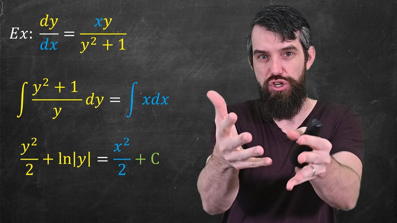
Separation of Variables // Differential Equations
5.0 / 5 (0 votes)