METODE BEDA HINGGA || METODE NUMERIK UNTUK MASALAH NILAI AWAL (BAGIAN II)

Summary

This video explains numerical methods for solving initial value problems using the finite difference method. It focuses on forward and backward schemes for solving differential equations, with an emphasis on the explicit and implicit methods. The tutorial covers how to implement these methods, highlighting the differences in the approaches and their practical applications. The video also discusses the importance of prediction and correction steps in the methods, and introduces the concept of a weighted average method for improved accuracy. Ultimately, the video provides viewers with a clear understanding of various finite difference methods and their implementation in mathematical modeling.

Takeaways

• 😀 The video continues the discussion on numerical methods for solving initial value problems using finite difference methods in mathematics.
• 😀 The initial value problem is introduced, where the problem may or may not depend on time. The focus is on solving problems that do not depend on time.
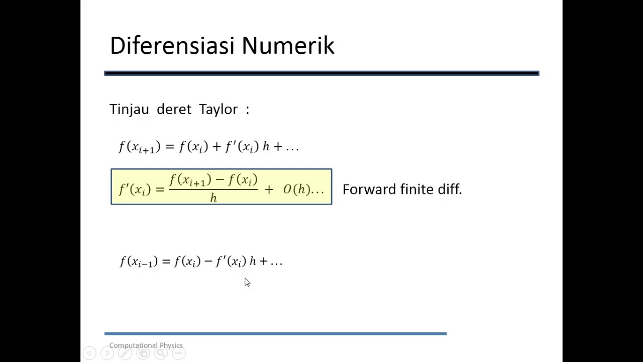
• 😀 The forward difference method, or 'explicit method,' is explained, which approximates the derivative using the difference between values at adjacent points in time.
• 😀 The concept of forward difference is illustrated with a graphical representation of the first derivative of a function, highlighting the change over time.
• 😀 The backward difference method, or 'implicit method,' is introduced, which requires the value at the next time step to be calculated from the current one.
• 😀 The backward difference method is explained as requiring both predictor and corrector steps, where initial predictions are refined using the implicit method.
• 😀 The explicit method is considered less stable compared to the implicit method because it only uses current values, which can cause instability in certain situations.
• 😀 A comparison is made between the explicit and implicit methods in terms of their computational approach, with explicit methods using current values and implicit methods needing both previous and next values.
• 😀 The video then explains the method of averaging between forward and backward schemes to create a new method, providing a better balance between accuracy and stability.
• 😀 The Teta method, an extension of the previous methods, is introduced, allowing flexibility in choosing the weight between forward and backward schemes for better control over numerical results.

Q & A

What is the primary focus of the video script?

The primary focus of the video is on explaining numerical methods for solving initial value problems in differential equations using finite difference methods, particularly forward and backward methods, and an implicit method known as the backward method.

What is the finite difference method?

The finite difference method is a numerical technique used to approximate solutions to differential equations by discretizing the continuous problem into a system of algebraic equations. It replaces derivatives with finite differences to solve differential equations.

How does the forward method work?

The forward method is an explicit numerical scheme where the future value of the function is calculated using known values of the current and previous time steps. It is straightforward but can be less stable for stiff differential equations.

What is the backward method, and why is it considered implicit?

The backward method is an implicit numerical scheme where the future value of the function is used to calculate the solution. It is considered implicit because it requires solving a system of equations at each step, making it more stable, especially for stiff equations, but also more computationally intensive.

Why is the backward method more stable than the forward method?

The backward method is more stable because it incorporates information from the future time step, which helps to control errors and prevent instability, especially for stiff equations. In contrast, the forward method only uses the current and previous time steps, making it less stable in some cases.

What is the average method, and how does it combine the forward and backward methods?

The average method is a hybrid scheme that averages the results of the forward and backward methods. This method combines the simplicity of the forward method with the stability of the backward method, offering a balanced approach to solving differential equations.

How is the forward method evaluated in the context of the script?

In the forward method, the future value of the function is predicted using the values from the current and previous steps. The script defines this method in terms of finite differences, where the difference between successive values is divided by the time step, Δt.

What does the script mention about the computational complexity of the backward method?

The backward method is more computationally expensive than the forward method because it requires solving a system of equations at each time step. This makes it more stable for stiff problems but requires more computational resources.

What is meant by 'implicit' and 'explicit' methods in numerical analysis?

In numerical analysis, an explicit method computes the future value directly from the current and previous values, making it simpler but potentially unstable. An implicit method, on the other hand, uses future values in its calculations and requires solving an equation at each step, making it more stable but more computationally demanding.

What is the significance of the 'teta method' discussed in the video?

The teta method is a hybrid numerical method that combines the forward and backward methods. It introduces a parameter (teta) to adjust the weighting between the forward and backward methods, providing flexibility in how the scheme behaves. This allows for tuning the method between explicit and implicit schemes based on the value of teta.