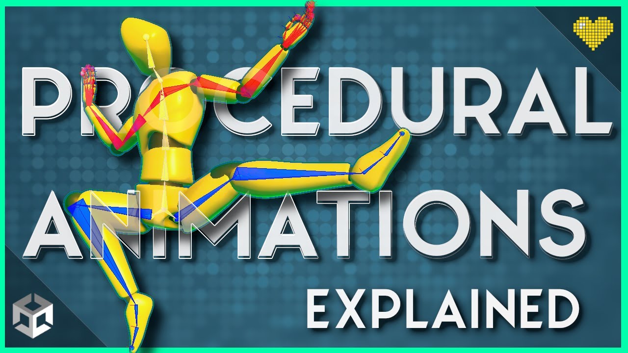
Giving Personality to Procedural Animations using Math
Summary
TLDRThis video delves into the fascinating world of procedural animation, contrasting it with traditional vector animation techniques. It explores how animators can create dynamic, responsive characters by utilizing concepts like inverse kinematics and second-order motion systems, represented by parameters such as natural frequency, damping, and initial response. The presenter demonstrates real-time applications in game design, discussing stability challenges and potential solutions. By modulating motion parameters based on gameplay context, developers can enhance character movement, conveying nuanced states of awareness and engagement. Overall, the video offers valuable insights into blending mathematics and art in animation.
Takeaways
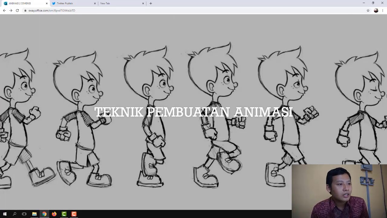
- 😀 Interpolation curves in traditional animation control motion dynamics like easing in and out, enhancing artistic expression.
- 🤖 Procedural animation in games allows characters to respond dynamically to input without relying on keyframes.
- 📏 The relationship between input and output in procedural animation can be modeled with variables for velocity and acceleration.
- 🛠️ A second-order system is a common approach in mechanical motion, where forces act on acceleration as per Newton's second law.
- 🎛️ Key parameters like natural frequency (f), damping coefficient (zeta), and initial response (r) can control motion characteristics.
- 🔄 The step response visualizes how a system reacts to sudden changes, capturing its dynamics effectively.
- ⚖️ Stability in feedback systems is crucial; instability can occur if the time step is too large relative to the system's parameters.
- 📊 The state-space representation helps analyze how state variables influence each other over iterations, ensuring system stability.
- ⏱️ A critical time step can be computed to prevent catastrophic failures during game execution, especially under variable frame rates.
- 🌐 Using parametric motion models can convey gameplay information, allowing for dynamic character movement based on various states.
Q & A
What are interpolation curves in traditional vector animation?
-Interpolation curves define how movement transitions between keyframes, allowing for effects like easing in and out, overshooting, and providing artistic control over motion dynamics.
What is the primary advantage of procedural animation in games?
-Procedural animation allows characters to adapt dynamically to changing gameplay situations without relying on predefined keyframes, enhancing realism and responsiveness.
How does the relationship between input (x) and output (y) function in procedural animation?
-The system aims to produce output (y) that tracks input (x) but incorporates additional dynamics to convey motion characteristics, rather than strictly conforming to input.
What are the roles of the parameters f, zeta, and r in controlling motion dynamics?
-Parameter f controls the natural frequency of the system, zeta (ζ) determines the damping behavior and how the system settles, while r influences the initial response speed to changes in input.
What is Euler's method, and how is it used in real-time animation?
-Euler's method is a numerical technique used to update position and velocity estimates iteratively during gameplay, based on the time elapsed between frames.
Why can high resonant frequencies lead to instability in a procedural animation system?
-If the resonant frequency (f) is set too high relative to the frame rate, it can cause the system to accumulate errors, leading to instability and potentially catastrophic behavior.
What is the significance of the state-space representation in analyzing motion stability?
-The state-space representation allows for organizing state variables in a matrix form, facilitating the analysis of stability through eigenvalues, which helps ensure the system remains stable over time.
How can parameter modulation enhance gameplay experience?
-By modulating parameters like f, zeta, and r based on character states (e.g., health or awareness), developers can create more nuanced and responsive animations that communicate gameplay information to players.
What is critical damping, and how is it applied in animation?
-Critical damping occurs when zeta equals 1, causing the system to settle quickly without oscillating. It's used in Unity's SmoothDamp function to achieve smooth and responsive movements.
What additional techniques can be employed to improve accuracy in fast-moving procedural animations?
-Techniques like pole-zero matching can be implemented to compute k1 and k2 values dynamically per frame, enhancing accuracy during rapid movements at the cost of increased computational demand.
Outlines

This section is available to paid users only. Please upgrade to access this part.
Upgrade NowMindmap

This section is available to paid users only. Please upgrade to access this part.
Upgrade NowKeywords

This section is available to paid users only. Please upgrade to access this part.
Upgrade NowHighlights

This section is available to paid users only. Please upgrade to access this part.
Upgrade NowTranscripts

This section is available to paid users only. Please upgrade to access this part.
Upgrade NowBrowse More Related Video


5.0 / 5 (0 votes)