A primer to wireless power transfer

Summary

La présentation intitulée 'A primer to wireless power transfer' explore l'idée de la transmission de puissance sans fil, une notion ancienne popularisée par Nikola Tesla en 1898. Le texte décrit le concept de base impliquant des bobines primaires et secondaires, la création de flux magnétique et le coefficient de couplage qui détermine l'efficacité de la transfert. L'auteur aborde les défis, notamment la distance, les pertes par résistances parasitaires et la question de la puissance apparente. Il insiste sur l'importance des circuits résonants pour améliorer le couplage et explique le rôle du facteur de qualité (Q) dans ces circuits. La présentation couvre également divers modèles de circuits, y compris les équivalents de résistances pour des charges non linéaires telles que des batteries. Enfin, elle examine les méthodes pour améliorer le découplage et augmenter le coefficient de couplage, comme l'utilisation d'éléments de ferrite pour canaliser les lignes de flux. L'objectif est d'offrir une vue d'ensemble intuitive du transfert de puissance sans fil, soulignant sa complexité et la nécessité d'une adaptation aux différents types de charges pour obtenir des résultats optimaux.

Takeaways

• 🕰️ L'idée de transfert d'énergie sans fil n'est pas nouvelle, remontant à Nikola Tesla en 1898.
• 🔌 Le transfert d'énergie sans fil a été exploré dans les années 1920, avec des suggestions de constructions de transformateurs sans fil dans des journaux bricoleurs.
• 🌐 L'idée de Tesla visait non seulement à une technologie, mais aussi à une foi et une idéologie pour améliorer les relations pacifiques universelles en éliminant la distance.
• 🪢 Le coefficient de couplage est un facteur clé dans le transfert d'énergie sans fil, déterminant la quantité de flux magnétique atteignant le secondaire.
• ⚙️ Le modèle de système peut être basé sur la mutualité ou sur la relation d'un transformateur, avec des notions de permeabilité et de pertes.
• 🔋 L'efficacité du transfert d'énergie sans fil est cruciale, nécessitant une gestion des pertes et une réduction de la puissance apparente.
• 🔗 L'utilisation de circuits résonnants est une approche pour améliorer le couplage entre les bobines et réduire l'impédance totale du circuit.
• 📡 Le facteur de qualité (Q) est important dans les circuits résonnants, influençant la forme de l'onde sinusoïdale et la relation entre l'énergie réactive et réelle.
• 🔧 L'efficacité du transfert peut être optimisée en réduisant les pertes dues aux résistances parasitaires et en utilisant des composants à faible résistance équivalente série (ESR).
• 🔄 La simulation de circuits peut aider à comprendre le comportement du système sous différentes conditions et à trouver les points de fonctionnement optimaux.
• 🛠️ Il existe différentes configurations pour le transfert d'énergie sans fil, y compris des résonances séries et parallèles à l'entrée et à la sortie, chacune ayant ses avantages et inconvénients.

Q & A

Quelle est la première mention de la transmission sans fil de l'énergie ?

La première mention de la transmission sans fil de l'énergie a été publiée par Nikola Tesla en 1898.

Quel était le but initial de la transmission sans fil de l'énergie selon Tesla ?

Selon Tesla, le but initial de la transmission sans fil de l'énergie était de contribuer à des relations pacifiques universelles par l'élimination de la distance.

Comment la capacité électronique moderne influence-t-elle la transmission sans fil de l'énergie ?

La capacité électronique moderne rend la transmission sans fil de l'énergie beaucoup plus pratique grâce à l'amélioration de la technologie.

Quel est le facteur clé dans la transmission sans fil de l'énergie ?

Le facteur clé dans la transmission sans fil de l'énergie est le coefficient de couplage, qui détermine la quantité de flux magnétique généré dans le bobinage primaire et qui parvient au bobinage secondaire.

Comment les circuits résonnants améliorent-ils la transmission sans fil de l'énergie ?

Les circuits résonnants améliorent la transmission sans fil de l'énergie en augmentant le coefficient de couplage entre les bobines et en réduisant l'impédance totale du circuit.

Quelle est la définition du facteur de qualité (Q) dans un circuit résonnant ?

Le facteur de qualité (Q) dans un circuit résonnant est défini comme le rapport entre l'énergie réactive et l'énergie réelle, ce qui indique l'efficacité énergétique du circuit.

Quels sont les défis dans la transmission sans fil de l'énergie ?

Les défis dans la transmission sans fil de l'énergie incluent la distance, qui affecte le coefficient de couplage, les pertes dues à la résistance parasitaire, et la gestion de la puissance apparente.

Comment l'efficacité de la transmission sans fil de l'énergie est-elle définie ?

L'efficacité de la transmission sans fil de l'énergie est définie comme le rapport entre la puissance de sortie et la puissance totale entrante, qui inclut les pertes dues aux résistances parasitaires.

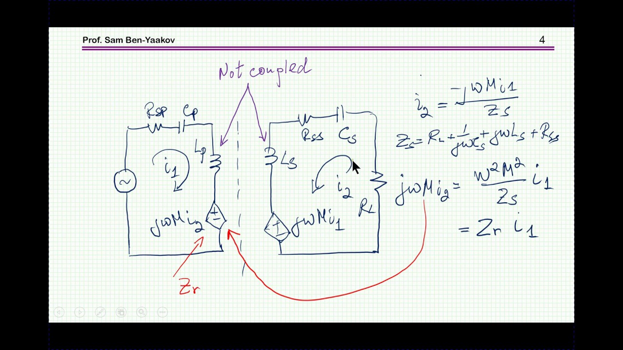
Quels sont les avantages de l'utilisation de l'inductance mutuelle dans un modèle de transmission sans fil de l'énergie ?

L'utilisation de l'inductance mutuelle permet de modéliser la dépendance du courant secondaire en fonction du courant primaire, ce qui simplifie l'analyse et la compréhension du transfert d'énergie.

Quels sont les éléments à prendre en compte pour optimiser la transmission sans fil de l'énergie ?

Pour optimiser la transmission sans fil de l'énergie, il est important de réduire les pertes dues à la résistance, d'utiliser des condensateurs à faible ESR (résistance série équivalente), et d'adapter la configuration du circuit en fonction de la résistance de charge.

Comment la simulation peut-elle aider dans l'analyse de la transmission sans fil de l'énergie ?

La simulation peut aider à comprendre le comportement du circuit sous différentes conditions, à identifier les points d'optimisation et à prédire les performances du système en fonction des différentes configurations et paramètres.

Outlines

00:00

🔌 Présentation du transfert de puissance sans fil

Sabine Yaakov introduit le concept de transfert de puissance sans fil, une idée ancienne popularisée par Nikola Tesla en 1898. Il a proposé un système de bobine primaire, de condensateur et de bobine secondaire pour créer une résonance et transférer de l'énergie. Plus tard, en 1921, un article a suggéré une expérience de transfert de puissance sans fil à l'aide d'un transformateur. Aujourd'hui, avec les avancées électroniques, le transfert de puissance sans fil est plus pratique. Tesla voyait cette technologie comme un moyen d'unifier la distance et promouvoir des relations pacifiques universelles.

05:01

🔗 Principes du transfert de puissance sans fil

Le transfert de puissance sans fil repose sur le concept de couplage entre deux bobines. L'énergie est transférée par le flux magnétique créé par une bobine primaire alimentée en AC. Le couplage efficace est déterminé par le coefficient de couplage, qui est une mesure de la quantité de flux magnétique atteignant la bobine secondaire. Les modèles de mutualité inductrice et de transformateur sont utilisés pour modéliser le système. Le but est de transférer autant de puissance que possible de manière efficace, en tenant compte des pertes dues à la résistance parasitaire et de l'importance de réduire la puissance apparente pour minimiser les pertes et les besoins en composants réactifs.

10:01

🎵 Circuits résonants et facteur de qualité (Q)

Les circuits résonants série et parallèle sont essentiels pour améliorer le couplage entre les bobines. Ils permettent de réduire l'impédance totale du circuit en résonance, permettant ainsi un transfert de puissance plus efficace. Le facteur de qualité (Q) est un indicateur de l'efficacité énergétique du circuit; un Q élevé signifie une forme sinusoïdale du courant, ce qui est souhaitable pour la commutaison de courant zéro. Cependant, un Q trop élevé peut nécessiter des éléments réactifs plus grands et augmenter les pertes. Les paramètres clés comme la fréquence de résonance, l'impédance caractéristique et le Q sont discutés, ainsi que leur importance pour le transfert de puissance sans fil.

15:05

🛠️ Simulation et efficacité du transfert de puissance sans fil

Pour comprendre le comportement du transfert de puissance sans fil, des simulations sont effectuées avec des circuits modèles. Les simulations AC et en temps réel sont utilisées pour observer les performances du système sous différentes conditions. Les résultats montrent que la fréquence de résonance et l'efficacité du transfert de puissance peuvent varier en fonction des composants et de leur configuration. L'efficacité est mesurée en comparant la puissance à la sortie avec la puissance fournie à l'entrée, en tenant compte des pertes dues à la résistance parasitaire.

20:07

🔍 Analyse et ajustement des composants pour l'optimisation

L'analyse des simulations révèle que la résonance et l'efficacité du transfert de puissance sans fil sont influencées par l'interaction entre les composants du circuit. L'ajustement des valeurs des composants, tels que les bobines et les condensateurs, est essentiel pour atteindre une résonance optimale et une efficacité maximale. Il est également important de considérer la résistance de charge et de s'assurer que la configuration du circuit est adaptée au type de charge, comme une batterie, pour obtenir les meilleurs résultats.

25:09

🔄 Configurations de résonance pour le transfert de puissance sans fil

Il existe différentes configurations de résonance possibles pour le transfert de puissance sans fil, notamment série et parallèle à l'entrée et à la sortie. Chaque configuration présente des avantages et inconvénients en termes de puissance apparente, de courant et de contrôle. Par exemple, une résonance série à l'entrée peut générer une forte puissance apparente et un fort courant, tandis qu'une résonance parallèle à la sortie peut réduire le courant qui passe à travers les composants. Le choix de la configuration dépend des exigences spécifiques de l'application.

30:10

🛑 Conclusion et amélioration du transfert de puissance sans fil

La présentation conclut en identifiant les défis et les opportunités associés au transfert de puissance sans fil. Il est important de sélectionner les composants et la configuration du circuit en fonction des besoins spécifiques pour obtenir une efficacité et une performance optimales. Des méthodes pour améliorer le couplage et augmenter le coefficient de couplage, tels que l'utilisation d'éléments de ferrite, sont discutées. Ces méthodes peuvent aider à optimiser le transfert de puissance et à surmonter les défis techniques associés.

Keywords

💡Transfert de puissance sans fil

Le transfert de puissance sans fil est le processus de transmission d'énergie électrique à distance sans le recours à des connexions électriques physiques. C'est le thème central de la vidéo, expliquant comment l'énergie peut être transférée à travers l'air à l'aide de la technologie basée sur l'induction magnétique. Dans le script, cela est abordé en détail, y compris les défis tels que la distance et l'efficacité.

💡Nikola Tesla

Nikola Tesla est un inventeur et scientifique serbe qui a contribué de manière significative au domaine de l'électricité et des communications sans fil. Dans le script, il est mentionné comme étant le premier à publier l'idée de transfert de puissance sans fil en 1898, faisant de lui une figure clé de l'histoire de cette technologie.

💡Boucle primaire et secondaire

Les boucles primaires et secondaires sont des éléments essentiels des systèmes de transfert de puissance sans fil. Elles sont des enroulements de fil qui créent un champ magnétique résonnant pour transférer de l'énergie. Dans le script, leur rôle est décrit dans le contexte de la création d'un flux magnétique et de la génération de voltage pour le transfert de puissance.

💡Coefficient de couplage

Le coefficient de couplage (K) est une mesure de l'efficacité de la transmission d'énergie entre la boucle primaire et la boucle secondaire. Plus le coefficient est élevé, meilleure est l'efficacité de la transmission. C'est un concept clé abordé dans le script pour expliquer la quantité de flux magnétique qui atteint la boucle secondaire.

💡Résonneurs

Les résonneurs sont des composants utilisés pour améliorer le couplage entre les boucles primaires et secondaires dans un système de transfert de puissance sans fil. Ils sont décrits dans le script comme des circuits séries ou parallèles qui peuvent être ajustés pour maximiser la fréquence de résonance et l'efficacité de la transmission d'énergie.

💡Fréquence de résonance

La fréquence de résonance est la fréquence à laquelle un circuit résonnant fonctionne avec le maximum d'efficacité. Elle est cruciale pour le fonctionnement optimal des systèmes de transfert de puissance sans fil. Le script explique comment cette fréquence affecte le comportement des circuits résonneurs et la capacité de transfert d'énergie.

💡Impédance caractéristique

L'impédance caractéristique est une mesure de l'opposition au courant dans un circuit résonnant. Elle est déterminée par le rapport carré de la valeur de l'inductance à la capacité. Dans le script, elle est mentionnée comme un facteur clé pour comprendre les performances des circuits résonneurs.

💡Facteur de qualité (Q)

Le facteur de qualité (Q) est un indicateur de l'efficacité énergétique d'un circuit résonnant. Un Q élevé signifie que le circuit est capable de stocker de l'énergie sans pertes. Le script discute de l'importance de maintenir un Q raisonnable pour un fonctionnement optimal et des implications de Q élevé sur la taille des éléments réactifs.

💡Perte de puissance

La perte de puissance est l'énergie qui est perdue dans un circuit en raison de la résistance et d'autres facteurs. Dans le contexte du transfert de puissance sans fil, minimiser ces pertes est essentiel pour assurer un transfert d'énergie efficace. Le script décrit les différentes sources de pertes, y compris la résistance parasitaire et l'effet de la distance.

💡Éléments réactifs

Les éléments réactifs, comme les inductances et les capacités, sont utilisés pour stocker de l'énergie dans un circuit et sont essentiels pour le fonctionnement des systèmes de transfert de puissance sans fil. Le script explique comment ils sont utilisés pour contrôler la fréquence et l'impédance du circuit pour maximiser l'efficacité de la transmission d'énergie.

💡Topologie de circuit

La topologie de circuit fait référence à la manière dont les composants sont connectés dans un système. Différentes topologies sont discutées dans le script, y compris les avantages et les inconvénients de chaque configuration, comme la résonance série et parallèle à l'entrée et à la sortie, et comment elles affectent la performance du système.

Highlights

L'idée de transfert de puissance sans fil n'est pas nouvelle, et la première indication de cette idée a été publiée par Nikola Tesla en 1898.

Le concept de transfert de puissance sans fil a été exploré et publié dans un journal pratique en 1921, montrant comment construire un système de transfert de puissance sans fil.

La capacité électronique moderne rend le transfert de puissance sans fil beaucoup plus pratique aujourd'hui que par le passé.

Le couplage entre les bobines est un facteur clé dans le transfert de puissance sans fil, déterminant la quantité de flux magnétique qui atteint la bobine secondaire.

La coefficient de couplage est une mesure de l'efficacité de la transfert de puissance, et il est affecté par la distance entre les bobines.

Les pertes dues à la résistance parasite et la puissance apparente sont des défis dans le transfert de puissance sans fil.

Les circuits résonants sont utilisés pour améliorer le couplage entre les bobines dans le transfert de puissance sans fil.

Le facteur de qualité (Q) est un paramètre très important dans les circuits de transfert de puissance sans fil, déterminant le rapport entre l'énergie réactive et l'énergie réelle.

Pour améliorer l'efficacité du transfert de puissance sans fil, il est important de réduire les pertes dues à la résistance parasite et d'utiliser des composants à faible ESR (résistance série équivalente).

Les simulations montrent que la fréquence de résonance et l'efficacité du transfert de puissance sans fil varient en fonction de la valeur des composants et de la résistance de charge.

L'efficacité du transfert de puissance sans fil dépend de la capacité à fournir une grande quantité de courant à la charge, ce qui nécessite un ajustement précis des composants.

Il est crucial de sélectionner la bonne fréquence de resonance pour maximiser l'efficacité du transfert de puissance sans fil.

La conception des circuits de transfert de puissance sans fil doit tenir compte de l'interaction entre les composants et de la complexité du système.

Des méthodes pratiques pour améliorer le couplage et augmenter le coefficient de couplage incluent l'utilisation d'éléments de ferrite pour canaliser les lignes de flux.

Les configurations de circuits comme les inverters résonants en push-pull parallèles sont utiles pour générer des courants résonants élevés sans surcharger les transistors.

L'utilisation de matériaux ferrimagnétiques peut augmenter le couplage entre les bobines et améliorer l'efficacité du transfert de puissance sans fil.

La présentation conclut en soulignant l'importance de l'adaptation des configurations de circuits et des composants pour répondre aux besoins spécifiques de chaque application de transfert de puissance sans fil.

Transcripts

hi I'm Sabine Yaakov this presentation

is entitled a primer to wireless power

transfer now the idea of wireless power

transfer is not new actually the first

indication of such an idea has been

published by Nikola Tesla in 1898 about

120 years ago and here it is if there's

a primary coil this is a capacitor for

actually creating your resonance here

this is a generator it's a secondary

coil and these are the output terminals

actually this was for it through

periodic a purpose for healing people

this has been very popular at that time

now later on this idea was actually

explored and here is a suggestion for an

experiment this is in a do-it-yourself

a journal of practical early electrics

and here they suggest how to build a

wireless power transfer this was

published in 1921

and here we have a transformer this is

the AC live this sparker generate pulses

high current pulses that go through this

resonant circuit and then we have the

secondary coil and lo and behold you

have a lamp which is connected and it'll

light when this will be in operation but

this is really not new however today of

course the electronics capabilities make

it much more practical now for Tesla the

idea of wireless power transfer was not

just a technology it was sort of faith

ideology because he was concerned about

universal peaceful relations and he

believed that this could be achieved by

an elation of distance and to achieve

this wonder alike

city is the one and only means okay well

this is a really very realistic and

unfortunately I don't think it

materialized as yet maybe in the future

now let's go back to ground this is a

very simple presentation of the wireless

power transfer we have a primary coil

which is excited by say an AC source if

the result there is a current here and

the magnetic flux is created and it's

getting all over the place now if I

teach me to put another coil close to it

then part of this flux k fraction will

enter this coil and will generate a

voltage and by this we'll get the

wireless power transfer because we have

power from here going through here to

here so okay it is really a very key

factor here this is the coupling

coefficient this is how much of the

total flux are generated in the primary

is actually reaching the secondary so if

we have a cake fraction at the secondary

and if the turns ratio is n 2 here and n

1 here we are going to get this voltage

ratio K times n2 to n1 which can be also

expressed as a square root of n 2 over L

1 obviously K is always smaller than 1

in a pro Chuan but it's really never 1

because there's always some flux which

is escaping

even if in a transformer which is wound

on a magnetic or ferrite core now they

wait to model a system like this

actually can go two ways one is use this

mutual inductance concept we have two

inductors

which are coupled here or we can use a

transformer record

diction here we have a transformer this

is a model of a transformer we have a

leakage at the primary a leakage at the

secondary this is the primary inductance

and this is now ideal transformer that

just accounts for the transfer ratio

between the voltage and the current so

there are actually two ways to go and in

fact in one occasion it would be easier

or better to use one model and in some

other applications or analysis it will

be easier to use this one so if we have

this mutual inductance between two coils

then this implies that at the primary

you have an inductor l1 is the original

inductor and then you have a dependent

voltage source which depends on the

current on the secondary this is the

current in the secondary with the mutual

inductance value here and the same thing

goes for the secondary you have any

dependent voltage source the magnitude

of which is J Omega M is the coupling

coefficient that I 1 if the current here

now am this coupling coefficient again

is a function of the coupling

coefficient this is most important

parameter in this situation and square

root of l1 times l2 now in the case of a

transformer and now I'm talking about a

one-to-one transformer because in many

application l1 and l2 are the same type

of the coil for inductors so for n equal

to 1 I can eliminate the ideal

transformer here because it's a

one-to-one and what I'm left with is the

two lesions and the inductance the

common inductance now this is reflected

to the primary then the leakage

inductance is l1 times 1 minus K change

the coupling coefficient if case 1 this

is the ideal case there is no

leakage and all that we see is this

common inductor okay we won and we see

l1 now is Cain becoming smaller and

smaller we see here larger and larger

leakage inductances and this inductor

however becomes smaller and smaller and

smaller see K times L 1 so if K is a

point 1 then we are left with a small

inductance here I in the case of a

one-to-one situation with the mutual

inductance we have similarly two

inductors which are the same in this

case and two voltage sources which again

are dependent on the current of the

other side so here it is here and here

it's a function of y1 so what's the

objective of wireless power transfer

trust before we like to transfer as much

power as we can this is of course the

purpose of the whole thing

and another one which is the key factor

in the efficiency like they do it that

it is highly efficient process as

possible now what are the problems that

are involved first of all the distance

small larger distance caused a small

coupling coefficient and therefore you

get only a fraction of the flux and

therefore you have somehow to handle the

fact that a lot of the flux is actually

being lost there is the issue of

parasitic resistances which are causing

losses and reducing the efficiency and

also there is the question of the large

apparent power this is the product of

voltage times M now you'd like this

product to be very close to the real

power because if this apparent power is

large it has many implications one of

them being the fact that you need larger

reactive element that is inductors and

capacitors because they have now to

store more energy another implication is

that you get a higher losses since

higher current will

pass through the swords so you'd like to

keep the apparent power as small as

possible now let me talk a little bit

about resonant circuits because we are

going to use this approach in order to

improve the coupling between the coils

so in this case we are talking about two

possible resonant circuits one is the

serious one here's the serious month and

see an artist's load positive resistance

if there is no load and here's the

parallel one LC in vomit and this is the

current source now there are key

parameters that we need to address the

circular resonant frequency 1 over

square root of LC the resonant frequency

Omega times 2 pi the characteristic

impedance the square root of L over C

now another key factor which is very

very important in the wireless power

transfer is the cube that is the quality

factor now for the series circuit its

defined as Omega L over R now notice

this is really the ratio between the

apparent of energy or reactive energy to

real energy because if you multiply it

by I square here and I square here this

will be the energy stored in the

inductor and the real energy now you'd

like you to be large on the one hand

because you'd like the circuit to have a

sinusoidal waveform this helps zero

voltage switching and some other

features however to logic the Q means

that this energy here is very loud so

you need large reactive element so we

like to keep Q really in a reasonable

range I'll talk about it in a second now

you can express the Q the quality factor

in this ratio 1 over Omega RC or the

characteristic impedance overarm now in

the case of the parallel circuit its

bring one over it will be R over Omega L

and we are over here now in this case in

the series case when R approaches zero

then you have a very high quality factor

in the parallel case when R becomes

infinity then you have a large Q factor

so these are the basic concept of a

series and parlin a regular number now

we can use now the resonant circuit in

order to reduce the total impedance in a

circuit now if we have a branch like

this and we are at resonance that the

total impedance here zero so when we

have here resonance we are going to see

from the source only R because these two

cancel each other the impedances okay

this one plus and minus and the same

thing goes here at resonance we're going

to see only R so we are going to use

this to our advantage in the case of the

wireless power transfer by adding

capacitance here now what would you like

to do that because otherwise we have an

inductance and this is actually limiting

the current that will be passing to the

output so by putting this inductor this

capacitor here I can and when working in

the proper frequency I can reduce the

convenience of this branch and allow

more current to go to the load so you

can see it over here and you can see it

here we had here this case two capacitor

notice that the resonant circuit are not

very clear here I mean I can talk about

these two but then we have this

inductance which is also currently

playing some role we'll talk about this

a little bit late

so in a very simplistic way you can say

that if you put a capacitor in you work

at resonance then you're going to see in

in this presentation of the transformer

a inductor K times L and RL and

obviously now part of the current we see

now it here is passing through here and

you are losing some of the primary

current so as K is becoming smaller and

smaller we have problem in transferring

of power to the load okay so we need a

high current same thing goes in this

representation of the mutual inductance

obviously here we have K the larger the

smaller decay the smaller is this

dependent voltage source and less power

will be delivered to the load so what

about the efficiency efficiency is the

output power over the total power that

coming from the input and the input has

to supply the output power plus all the

losses now in this circuit in this

equivalent circuit the losses due to

parasitic resistances and this include

first twofold the driver is that the

MOSFET are the asan resistors resistors

the induct day of positive resistance of

the inductor coils ESR equivalent series

resistance of the capacitor and the same

thing goes there

so the efficiency will be the ratio

between the real power I n is a

normalized I to 2 I 1 and divided by the

total actually power which is the this

is the contribution or the loss due to

the positive resistance of primary this

is the secondary and here is the so in

order to help or get high efficiency

you'd like to reduce

our L first of all and this could be

done by using whips wire so that the RAC

as it is called that is the resistance

at high frequency will still be very

acceptable you need a low ESR capacitors

and of course the driver should have a

lower these on transistors so that RS

this equivalent resistance or below let

me just point out that this circuit

although it looks very sort of it's

simple it is really complex because

there are many interactions here there

already mentioned this inductor here

plays a role in the resonance of the

secondary in primary and therefore a

complete analytical study of the circuit

is really complicated and it leads to

rather long equations this is not the

purpose of this presentation which is a

an intuitive look at the whole issue of

wireless power transfer just to get the

feeling of what's all about here let's

consider two cases let's start with this

gift this assume that me already is very

high and that representing it by an open

circuit well here you see we have

resonance now here there's nothing here

so the resonant frequency will be C 1

and the total which is by the way the

original primary inductance because this

Plus this is L ok and if you drive the

circuit at this resonant frequency you

get a very high voltage again more than

one I mean the ratio will be much more

than one and then if you have a high

resistance here you get quite a bit of

power so this is another this is another

mode of operation having a large

resistance here if the resistance

however is very small and I'm

representing it by short notice that we

have now here e so the vane Network

- super resonant Network and plus

another network it's a rather it's not a

simple circuit here and of course there

are many resonant Peaks that you can

detect it various frequencies so in

order to simplify the understanding of

this circuit I'm going to do some

simulation and present some of the

results just to show the behavior of the

circuit under various conditions and the

circuit I'm going to simulate is this

circuit two inductors which are equal

they're 86 microhenry with two capacitor

which I'm going to change later on there

is the AC source and I'm going to do two

type of analysis and AC analysis for

this you need an AC source and I'm going

to do also a time domain analysis a

transient allowances for this you need a

transient source of time domain source

and I've interviewed the people just to

fill it with a square wave if you would

do with the driver in a practical

circuit if the capacitor is not twenty

nine point forty five the resonant here

is 100 kilohertz the Karthik impedance

of this circuit is 64 oh and just for

the sake of the numerical analysis

because simulation made a miracle I'm

assuming a 10 million paralytic

resistance in the primary and at a

second so I'm going to do actually two

type of simulation one assuming that K

the coupling coefficient is 0.5 so this

will be sort of the equivalent circuit

that we considered is that point one

should be L here - and this is 0.5 and

then I'm going to use two capacitor 1 C

this is the capacitor dead for 100

kilohertz as the resonance for the whole

inductor and to see because to see

half L is giving a resonant in here okay

and then I'm going also to run a

simulation for K point one and we have

then this is point one and of the

original primary or common inductor and

this is actually approaching already L

okay so this is very small and these are

very large and I'm going to run it for

the 29 nano farad capacitor

okay here's the schematics of this

circuit there we are going to run let me

zoom on it so we can see it better here

we see the two inductors which are

coupled we have here the K linear the

element that is coupling L 1 and L 2

this is L 1 and L 2 there are 86 micro

Henry coupling coefficient is 500 merely

that it's point 5 we have here two

sources one is an AC source it is before

an AC and all these small signal

analysis and then we have a pulse type

source it's a plus/minus amplitude and

with some rise time of 0.1 microsecond

and the pulse width and period are

adjusted so that the frequency will be

like in this Ferrari Qin see here it's

defined it 100 kilo Hertz we can change

it and the duty cycle will be one half

okay so the two capacitors are defined

by parameters this is just an initial

very we're going to change it and then

we have a resistor this is the load

resistor which is also defined here

before we're going to change it right

now and we have some parasitic

resistance here and here I've just

specified it to be

the milliohm so let's change this one to

say one owned to begin with and let's

see let's run the AC simulation let's

see what is actually if the setting here

a 10 kilo her to 300 kilohertz 1000

point three decades or have a good

resolution and we have a parameter

switch of C and I'm going to do a value

list and so these are two values this is

the twenty nine point four five a nanner

and sixty eight point nine and these

correspond the twenty nine is for this

resonance and the larger capacitor is

for the model in which for a coupling

coefficient of 0.5 we are going to have

the leakage it will be 0.5 of the

inductor so therefore we need a

capacitor which is twice as large okay

so let's start with this AC analysis let

me first of all have a look at the first

capacitor this is the twenty nine point

forty five nano and I have set up scales

as follows we have the inductor the

input current inductor current we had

the output voltage this is across the

load we have the power of the load to

the power and we have actually the

efficiency which is the power on the

load divided by the power that comes off

are the source okay now the now this is

for let's remember one own load and the

capacitor is a twenty nine so that the

resonant is between supposed to be

between the total inductance and

capacitor what we observe here is really

much different to begin with we see two

peaks one it this will be one a little

bit over 140 kilo Hertz and this one is

a little bit over 80 kilo Hertz there

are two pics here this is the say the

output and of course you see the current

at the input okay so we had sort of a

split phenomenon in which the supposedly

one resonance is split into two and

again this is because there is an

interaction between all the components

in the system okay and if we look at the

output we see that we have a fairly high

output remember I didn't mention it but

the excitation is one volt

okay one bull so we have a one volt

output is about one volt and the power

is a little bit less I don't know why

supposed to be one what maybe there is a

difference here between peak and RMS

values I am not so sure so then we look

here at a this is sort of an efficiency

we see the efficiency is fairly high

remember we have pathetic resistances of

50 milli ohms below this one ohm so

relatively the losses are not that high

interesting enough we have another peak

here for high efficiency and this pig

indeed is at 100 kilohertz

okay but this peak is at the point this

is virtually no output over let me say

that the output is very very small okay

and

then the input is small and the ratio

between them and is pretty good but this

is not a useful point so the conclusion

here is that for one owned with this

capacitor we have two peaks and

frequencies which are different from

this one kilo Hertz and we get a pretty

good transfer function with this 0.5

coupling coefficient let me now go back

and have a look at the situation for the

fifty eight point nine nine afraid okay

I'm selecting at this value and well the

picture is not much different except

that the old frequencies actually

shifted downward lo and behold we have

now a peak and 100 kilohertz there's a

peak here we have a a peak current at

the input we have a peak output voltage

and then we have a good efficiency but

then we have another peak at a much

lower frequency this is supposed to be

the b-17 above sixty close to 60 akira

hurt there's another peak and for this

peak we get also a pretty good result

however this high efficiency is really

useless because at this point we just

don't have any output and of course

there is no input okay so this is the

situation with the capacitor which is

twice as big so that the resonant is

between the capacitor and a half the

inductor half decide the value of the

inductor let me now move to the case of

a different resistor and let me put this

month to be like

27 oh you remember that the

characteristic impedance of this circuit

calculated just by this inductor and

this capacitor which really doesn't tell

the whole story but if you use these to

calculate the characteristic impedance

it comes out to be 54 so we are now at a

value which is like half so wailing

supposedly having formerly a queue of

two okay so let's run this one now and

I'll pick the first one and wow we have

a whole different story here and you can

see the sort of q2 is causing this

circuit to look very flat this is the

efficiency it's very high here but again

one has to look at the output but

unfortunately the output as far as the

power goes is not very good indeed we do

get a fairly high output voltage about 1

that is we have actually again above the

input but since the resistor now is much

larger it's 27 as compared to 1 then

obviously this square over R which is

the power is now much lower and indeed

we having only like 50 millivolts so we

have a problem here in terms of the

amount of power that we are delivering

but not again that this flat behavior

that kind of suggests low Q circuit now

let me now go back and change the

resistance even further let's make it

let's say 100 ohm and run it again and

we'll choose again this 1929 Nana all

right well we have a different story

here we have one resonant one resident

and it is at

100 kilohertz this is because we have

now our rhythm and this is like an open

circuit at the output which are shown

earlier one of the slides so we really

have a resonant between the whole

conductor and the capacitor and we know

this should be at 100 kilohertz and

indeed it is we have a output which is

fairly high because the Q is high and

this is now like a parallel circuit

partially and we have a higher voltage

but still the amount of power that we

get out is not very much is only 120 250

a millivolt at this point however the

efficiency is furthering high because

now we have a much larger load resistor

as compared to the 50 million of the

parasitics then of course the efficiency

will be high okay that's do even larger

make a larger registered say 1 kilo ohm

and then of course we are just about a D

and this is indeed like a open circuit

the Q is much higher now like a parallel

circuit and the output voltage is much

higher see that we get a much higher

voltage we do have now a fairly high

output power this is above 1 watt and

this is because the voltage is 3 hi and

so that this 40 squared less

thirtysomething divided by 1 kilo ohm is

again 1 what now the input current in

this case is not that high it's about 1

ampere it's a little bit more than one

end

and one amp would be the power required

for one one and this is a little bit

higher so we see that the VA the

apparent power is is not that high as

far as the input source is concerned so

what really this teaches us that the

situation is really complex and you have

to look at your particular load resistor

and match it to the configuration of the

circuit to get an optimum result

let me move now to the case of the 200

mini for the coupling coefficient that

is point to a K of point two and let's

start off with say again and one ohm

here and we see pretty much similar

situation maybe the frequencies that are

a little bit different you see these two

peaks are a closer one to another again

we have this strange high efficiency

point with no output power but the

situation is not very different and just

for a check

let's have a look at say 10 10 ohms here

what is happening okay now obviously

this total apparent quality factor is

worse these two peaks are sort of

getting closer and as you see here the

minimum now is not zero it's going up

and we get the same gain just about the

same gain however since the load

resistor is much higher to ten times

higher than the power is about ten times

lower so we get good efficiency but the

power output is low so the conclusion

here again is that you really have to

tailor the load to the particular

circuit and there's no one solution for

all loads let us now look at the

a transient responded if the time domain

remember we have here a square wave or

excitation so I'm moving to a transient

setting and let's see what is the

setting here we are running it for five

millisecond collecting data after 4.95

millisecond this is the resolution and

the parametric's which is again these

two capacitors I'm now back at the AC

the result of the AC analysis and the

reason is that I like to select the

operating point so let's start with this

100 kilohertz which is right here this

doesn't seem to be the optimum point but

this let's just see what's going on here

and now running it and this is for a

frequency of 100 kilohertz

okay let's choose again the twenty nine

point forty five nano farad and here it

is and this is now the output voltage

and you can see if you see a nice

sinusoidal waveform this is the

excitation this is the current of the

input and here we have the actual power

this is the product of the current times

the voltage on the load resistor okay

and average so this is now the power

which is not very good okay so let's go

back to the AC analysis again and run

the same one this is the AC analysis

again and let's run the 100 ohm case

again and the purpose of which would be

to find the frequency okay so I'm

turning on the cursor and let's have a

look at here look at

frequency and this is 110 point 63 let's

say 111 actually 111 kilo Hertz this is

this frequency okay so I'm returning now

to the circuit running a transient

analysis but changing it to 111 K and

running okay I'll choose the game this

29 rod and here what it is so we see

that the power is now higher we have an

ice on it so that waveform because of

the nice nicer Q so here we can examine

the actually time domain waveform of

this okay let's go back now to some real

circuits and see how we actually

implement this wireless power transfer

now this would be a very simple

realization we have here a half bridge

driven of course out with 180 degree

phase the phase shifted the pulses here

is the primary this is the secondary we

are talking about this resonant circuit

and we know that there are some

implication and questions but let's

leave these aside just look at the

circuit itself we have now a rectifier

and we have a smoothing or filter

capacitor plus RL bridge represent the

load now in the analysis we have been

using any resistor so it be useful to

replace this this is a nonlinear circuit

that you cannot use in AC analysis it

will be useful to replace it by an

equivalent and encourage our AC resistor

that is I like to replace this whole

thing by some resistor such that the

circuit will behave the same as far as

AC analysis goes now the way to do it

has been demonstrated many years ago by

professor

Steigerwald and the idea behind this for

presentation is to equate the power that

is you like to select a RAC such that

the power delivered to it'll consume

dissipated by it is equivalent to the

power dissipated by this DC current

through this RL load so here is the AC

side power this is the unknown yet

resistor this is the DC part okay now we

can now Express IDC as a function of I

RMS through the pic and the average

value 2 over pi and then from which we

get this RAC is it's about point eight

pi square is about 10 so it's point

eight correct so you can replace this

whole thing by by this and this is very

helpful when analyzing or simulating in

fact the circuit now there are some

other situations which are practical for

example if you are charging a battery

then you cannot represent this load by

airport this store it is a fixed voltage

and you may change the current so again

by equating these two power on the AC

power the DC we get this our AC

expression and in this case it is a

function well you can make it a function

of the DC current charging the battery

or the primary AC current so it's a

nonlinear resistor depending on the

operating point but for a given

operating point this is the value for a

given say charging of say if it is a

battery for point 4 volts 1 amp then

you'll get 3 point 6 ohm resistor our AC

equivalent attic when you for the

panelists another case is when you feed

the battery with the constant care

so this is a power type of shitload but

then again since you have the current

here and the battery is very similar to

what we had before so you end up with

something very similar as we had before

so this is the way to represent this

nonlinear of rectifier plus load by an

arrays looking now at the bigger picture

it turns out that this case of resonance

resonance at the input and output it's

just a private case of many other not

many but there are other possibilities

we can have a resonant search rather

than the input sir it's written on the

output we can have serious at the input

parlor at output and we have parlour the

input course should answer is it output

and of course Harlan and parlor now

what's the advantage and problem with

any of these connections now when you

have a serious resonant at the input you

have a fairly large apparent power and

you have all the current passing through

the source so the idea son of the

transistor sees all these cards it could

be high so in the output you have this

resistor in series with this resonant

circuit and obviously to get a

reasonable Q our L has to be smaller

than they characteristic impedance so

this leads to fairly low values of R

okay in this case in the second case

this would be suitable for loads which

are represented by a large arm so that

you can get a high Q at the secondary

given a certain value of characteristic

impedance of LHC and this again suffered

from the same thing here we have an

advantage in that we can generate a very

high current in the

resonant Network this here while this

current is circulating here and not seen

by the swords by the way for apartment

circuit this has to be a current source

because if it is a voltage source then

obviously you are imposing a voltage

here and the resonant doesn't take place

here at all so for a parallel resonant

primary unity current source secondary

again we have very serious and here

again we have part and pallet so this

will be helpful to eliminate the high

current through the coil from passing

through the input and here this is be

suitable for a high value of resistance

I mean high value compared to the

towards the convenience of the secondary

it can be concluded that the panel

connection at the input is really

desirable under all cases because it can

generate high current which is locked in

the parlour circuit not passing through

need and for the output it really

depends on the type of flow one way to

do it is to use this network shown here

this is the coil Primerica the input the

output coil and this is the inductor

should be very large and this is sort of

imposing current into this circuit as it

turns out that this circuit is really

not easy to control and also you cannot

very easily control the switching office

under all operating conditions so this

has not been used as far as I know it's

not been very popular another circuit

which is very interesting is a so called

push-pull parallel resonant inverter and

there are two configurations and I'll

start with this one which is the

original one and

being around for many years we have here

a parallel circuit for the resonant

circuit which is sent attempt okay and

then again we have a series resistor

these transistors are operated in 100

degree phase shift so that when this

pulse is high this is low and vice versa

when this voltage is high and this

transistor is conducting so this point

is connected to ground and since we have

the feed here

of the source then we start generating a

sinusoidal waveform of this at this

point they have the side this is ground

and this is the other side as we hit

this point this should be now pulled to

high voltage and clem this to ground and

then of course will start generating

hear a sinusoidal waveform going up like

here and again as you approach 0 will

change the situation and this is beyond

and this appeal so we need of course to

synchronize these two with the waveform

and we are going to have then

interleaving one side the other side etc

over the coil over the inductor we going

to have a sinusoidal waveform because we

have sinusoidal waveform half but they

have 180 degree to one side 100 nigiri

to the other side so we have a

sinusoidal waveform another

configuration is this one in here we

don't have a sensitive if it's not

convenient you don't want to have it we

have these two inductor which are

passing the DC current to this inverter

to power operation is very very similar

we have this sinusoidal waveform

generated as one side right Ron we have

it

other side etc so this is really a very

similar except for the fact that we

don't have this and the tab we paying

for it with two inductors instead now

it's interesting to realize that the

current that is passing through this

inductor hood through these inductor is

primarily DC current there's some ripple

depending on the size of that as large

as it will be the smaller larger will be

a less a smaller will be the ripple and

this this current times the voltage is

in fact just the read power coming off

the source so we have very little AC

current passing through the source and

which is a very desirable same thing

goes for these transistors these

transistors see only this current they

don't see this card this card is not

seen by this transistor arm in the

resonant current so you can build up a

fairly high resonant current without

this transistor passing it which is very

nice they are passing only this current

or this current okay this is the DC

current which are passed through the

transistor transistor do not see the AC

current which could be very high which

is very nice

finally let me say a few words about

ways to enhance our decoupling and to

increase the coupling coefficient and

one method that language has been shot

suggested is to end some ferrite

elements in the construction and this is

just one example there are many examples

that have been published practice here

we have the primary here we have the

secondary now we these are ferrite bars

okay a vector ferromagnetic bars ferrite

and what they do is actually the sort of

channel the flux to this direction

rather than the flux going all the way

to everywhere they are sort of

channeling it so if you place the

secondary coil the receiving coil sort

of around this of course they are bars

here too and just not showing it so

noise to confuse the picture so is this

secondary place over the primary it'll

capture these channel flux lines and

therefore it'll have a coupling

coefficient which is much larger than

you'd have without these apart okay so

this would be one way another way that

you need to put a plate of the

ferromagnetic material underneath and in

fact about okay so it'll lock the flux

in between that is that two different

weight and there of course the many

other ways to do this brings me to the

end of this presentation

hi thank you for your attention I hope

you have found it of interest and that

it will be useful to you in the future

thank you